Lesson two: Working with data tables

Welcome to lesson two: Working with data tables.

In the first lesson, we opened a workbook and placed a table element on the page from our connection to the Sigma Sample Database.

Now, we’ll manipulate this sample data table to make it an effective raw data source for our dashboard. By the end of this lesson, you’ll be able to independently transform the data in your table using sorting, filters, formulas, and more.

This lesson covers the following Sigma features:

• Table summaries
• Sorting
• Filtering
• Data types in Sigma
• Formulas in Sigma
• Hiding and organizing fields

The FAA sample dataset

For the rest of this course, we build on the FLIGHTS table as our data source. But before we can build it into a comprehensive dashboard, we need to understand the data inside the table, as well as our options for manipulating it.

Let’s familiarize ourselves with the sample data by exploring it using the basic functionality of tables in Sigma.

1. Open the Flight Delay Times workbook from lesson one for editing.

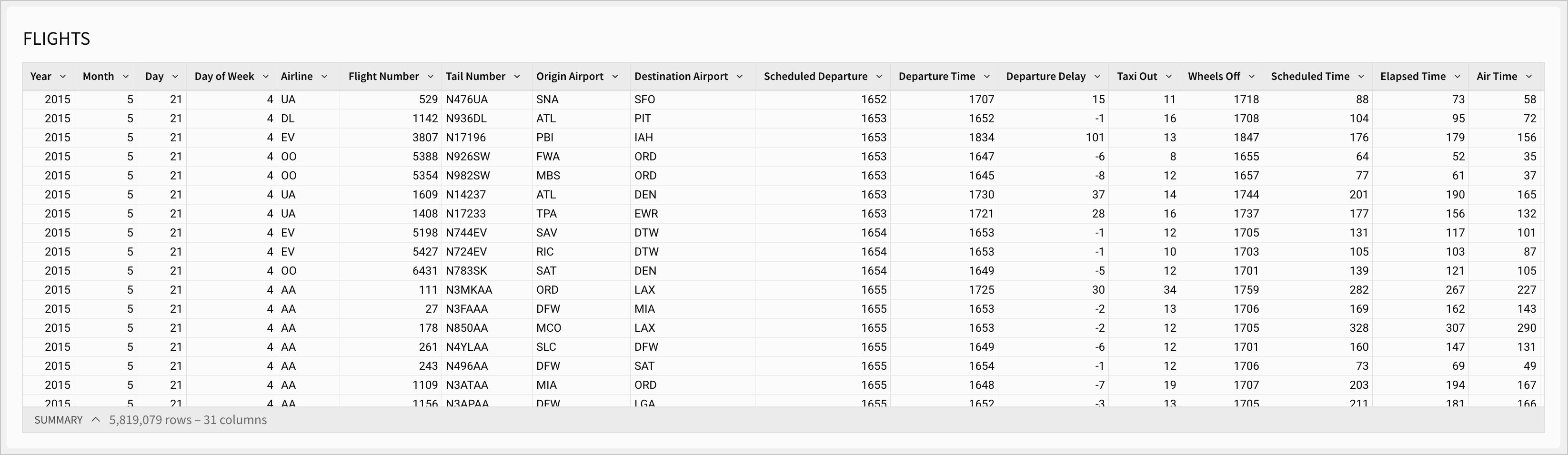
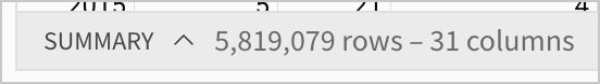
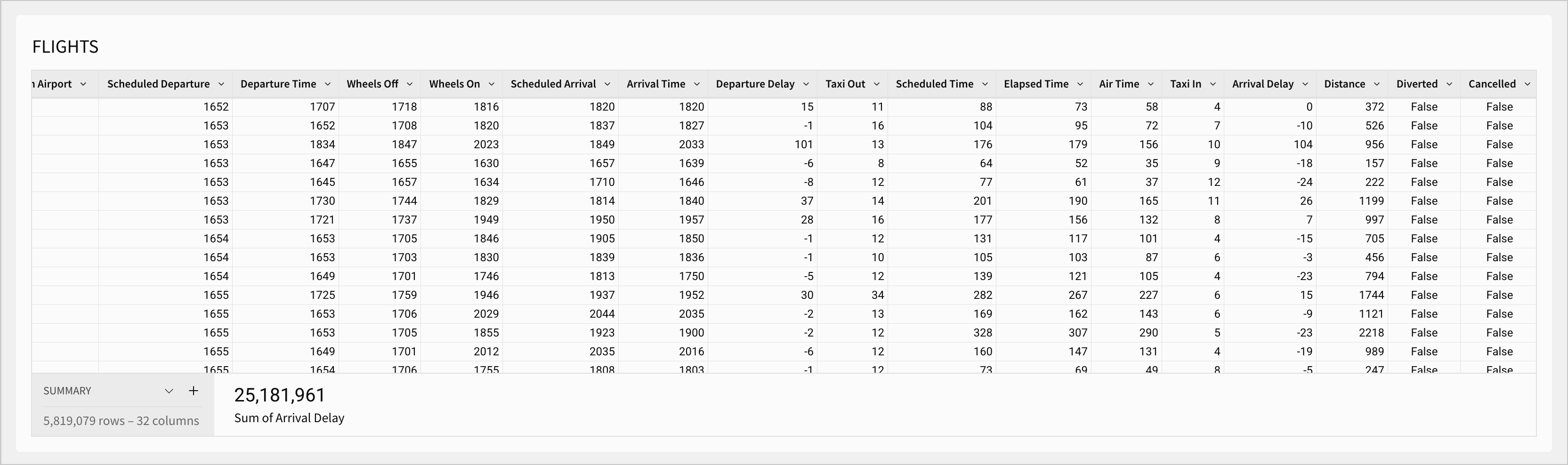
First, if we want to figure out how many rows and columns are in our table, we can look to the bottom-left corner, where the summary bar tells us the table has 5,819,079 rows and 31 columns. In the context of the FLIGHTS dataset, this means that we have data on 5.81 million individual flights, and for each flight we have 31 pieces of information.

Next, if we want to learn more about the columns in our table, we can look at the editor panel. When we have the table selected, the Properties section of the editor panel shows a column list with all 31 columns.

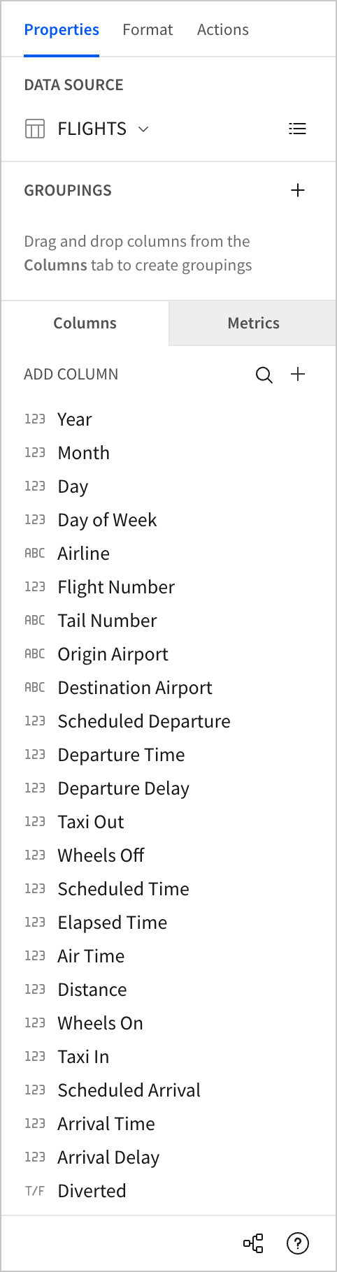
Each column is listed next to an icon that indicates its Sigma data type.

💡

Why does data type matter in Sigma?

Every column in Sigma is one of six data types: text, number, date, logical, variant, and geography. Data type determines which functions can be used on a column, as well as certain filter behavior.

For example, if you have a column of phone numbers that were automatically loaded into a column with the number data type, you might need to convert them to text to perform common operations, like filtering for 800 numbers. This is because filtering for phone numbers that start with 800 would require you to use functions like left and contains, which only accept text data.

Similarly, ZIP codes are often stored as text data in order to prevent the truncation of leading zeroes.

Let’s turn our attention to the data itself. Each record in this table is one US domestic flight from the year 2015, as recorded and reported by the Federal Aviation Administration. We see many fields we might expect to see in a table about flights, such as Airline, Flight Number, Origin Airport and Destination Airports, and more.

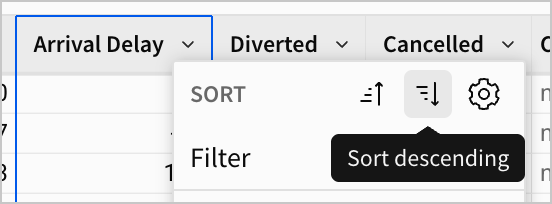
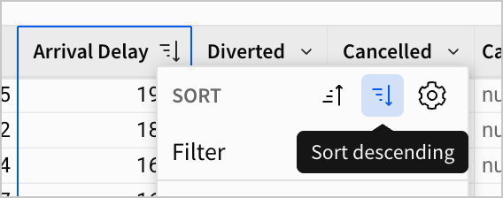
Each field has its own column menu, which we can open to see options to sort, filter, add new, and more.

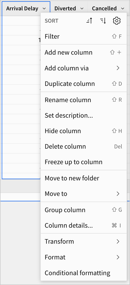
1. Open the column menu for the Arrival Delay column, and select Sort descending.

We now see the flights sorted from longest Arrival Delay to shortest. The flight with the longest Arrival Delay, for example, was delayed by 1971 minutes.

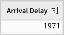
That’s a long delay - almost 33 hours in total. But this flight isn’t the only flight that arrived late. Let’s figure out how many total minutes flights arrived late by in 2015.

2. Back in the summary bar, click Show summaries for this table.

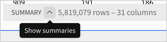
This reveals new options in the summary bar.

3. Click the Add summary… to create a new summary based on an aggregate of a column.

4. Select the Arrival Delay column from the Aggregate column menu, and a new summary titled Sum of Arrival Delay appears.

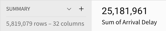
This has summed all the values in our Arrival Delay column - almost six million of them. It tells us that flights were delayed by a total of 25,181,961 minutes in 2015

💡

What if I want an aggregate other than sum?

You may have noticed that our summary automatically loaded as the Sum of Arrival Delay. This is because Sum is the default aggregate function for a number column in Sigma. You can change the aggregate by opening the summary menu, selecting Set aggregate, and picking a new aggregate.

Pay special attention to this when working with order numbers or other numeric ID columns. The default summary will return a sum of those values, even though ID numbers are not quantitative data. Aggregates like Count or CountDistinct are more appropriate for those types of data.

Transforming the data for our use case

For the rest of the lessons in this tutorial, imagine you’re an analyst at the FAA, tasked with creating a dashboard exploring flight delay times and their root causes using this dataset.

Our first step as an analyst would be to make sure we understand each column of our dataset, and then transform columns as needed to make our target analysis easier. Normally, this would be done by consulting a data dictionary, collaborating with the dataset’s owner, or getting context from an AI tool.

In the interest of time, the tutorial guides you to columns that need your attention. If you ever want to dive deeper into the details of a particular column, open the column menu and select Column details… to see summary information for that column.

First, let’s remove our sort from the Arrival Delay column.

1. In the FLIGHTS table, pan over to the Arrival Delay column.

2. Open the column menu, and reselect Sort descending to remove the sort.

The column is no longer sorted.

Now, let’s learn about the fields of our dataset. The first thing to notice is that there are several columns that represent time, and they all use the number data type. But despite using the same data type, these columns don’t all represent time the same way.

There are four types of columns that describe time in this dataset:

1. Columns that express a specific time of day:
   • Scheduled Departure
   • Departure Time
   • Wheels Off
   • Wheels On
   • Scheduled Arrival
   • Arrival Time
2. Columns that express an elapsed time in minutes:
   • Departure Delay
   • Taxi Out
   • Scheduled Time
   • Elapsed Time
   • Air Time
   • Taxi In
   • Arrival Delay
3. Columns that express a part of a date:
   • Year
   • Month
   • Day
   • Day of Week
4. Columns that express either an elapsed time in minutes, or a null value:
   • Air System Delay
   • Security Delay
   • Airline Delay
   • Late Aircraft Delay
   • Weather Delay

Let’s organize our columns to reflect these distinctions. Groups 3 and 4 are already grouped together in the data, but Groups 1 and 2 above are interspersed with each other.

By clicking on a column and dragging it, you can change its position in the table.

Drag and drop columns to separate specific times from elapsed times, like below:

Now that our data is visually organized into groups, let’s examine the individual columns. To start, let’s look at the columns that store a specific time to see how they’re representing it.

1. Open the column menu for Scheduled Departure column, and click Filter. This opens a number range filter.

2. For the minimum value, enter 1560. For the maximum value, enter 1599.

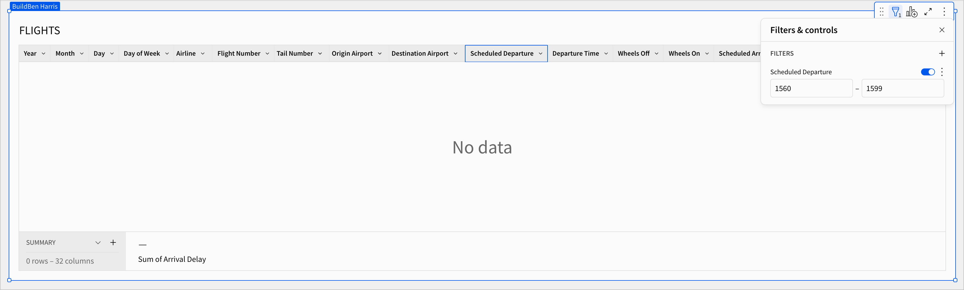
You’ll see that this filter leads to No data in our table.

This demonstrates that this column shows a specific time of day, where the value that comes after 15:59 would be 16:00. In time data, there are no values between 15:59 and 16:00. Similarly, in this number column, there are no values between 1559 and 1600 because the hour and minute as we read them on the clock have been combined into a four-digit number. Numbers like 1578 or 1593 don’t exist in the data as a consequence. However, this information is not stored as a time; it’s simply a number. Is this an appropriate way to store time data? What if a user tries to enter a value like 1578 or 1593? What time would that represent?

💡

Can I filter my data another way?

When applying a filter to a column with the number data type, Sigma creates a Number range filter by default. However, you can change filter type by selecting , selecting Change filter type, and choosing either List or Top N.

For example, if you’re working with a table that lists total sales for individual stores, you could use a Top N filter to show only the top 5 stores by total sales. If you wanted to select a specific set of stores to view, you could use a List with just their ID values.

Storing this time data as a number limits our future options. We can’t use functions that manipulate dates and times, and we can’t easily chart our data with a time dimension. We want to solve these problems now, so that our data is transformed for filtering, sorting, and visualization. Let’s use calculated columns and the formula bar to turn this number data into date data.

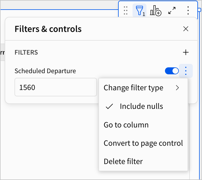
1. First, remove the filter from the previous step by opening the menu and selecting Delete filter.

2. Open the column menu for Scheduled Departure, and select Add new column.

This places an empty column, Calc, next to Scheduled Departure, and opens the formula bar at the top of the screen.

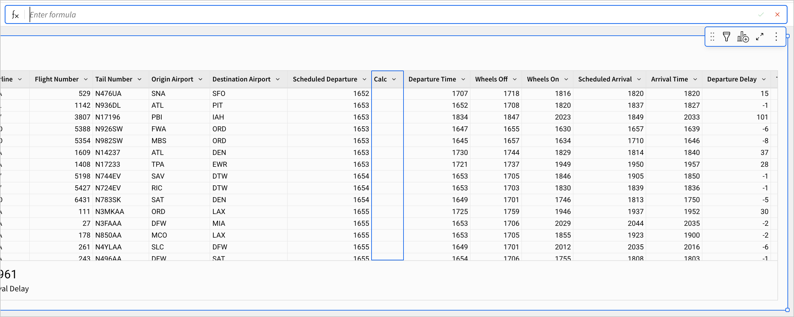
In the formula bar, we can use functions to create column-level calculations, dynamically populating each row with new data based on the formula we write.

Let’s look at a simple example of using a formula in Sigma. Consider the following entry to the formula bar:

Least(1, 2, 3, 10)

This formula uses a function called Least, which you can learn more about in the documentation.

Least accepts one or more arguments of the same data type, and returns the smallest value among them. In our example, it would return the value 1.

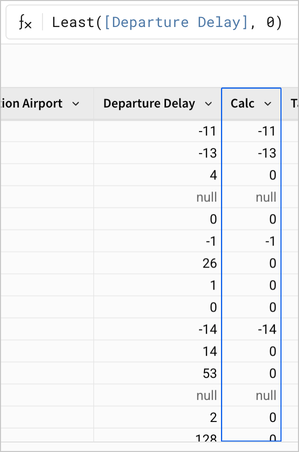
We can also reference columns in our function. Consider a second example: Least([Departure Delay], 0)

In this example, we are making a dynamic comparison for each row. If we add this formula to a new Calc column, like below, it returns the smallest entry between [Departure Delay] and 0 for each entry. This means that for negative Departure Delay values, it returns Departure Delay, and for positive values, it returns 0.

Notice that our dynamic reference, [Departure Delay], is enclosed in brackets. Otherwise, it’s treated like any other argument to the Least function. It is enclosed within the parentheses for Least, and is separated from 0 by a comma.

💡

How do I find functions?

When writing formulas in Sigma, functions are essential. Finding and implementing them is critical to transforming data.

There are two great self-service resources available for writing functions.

• You can find all available functions by category in the [doc:function-index).

• Additionally, your organization may have the AI formula assistant available, which can help turn written instructions into a formula.

Having reviewed a simple example of formulas and dynamic references, let’s write a formula that transforms our sample data for future use.

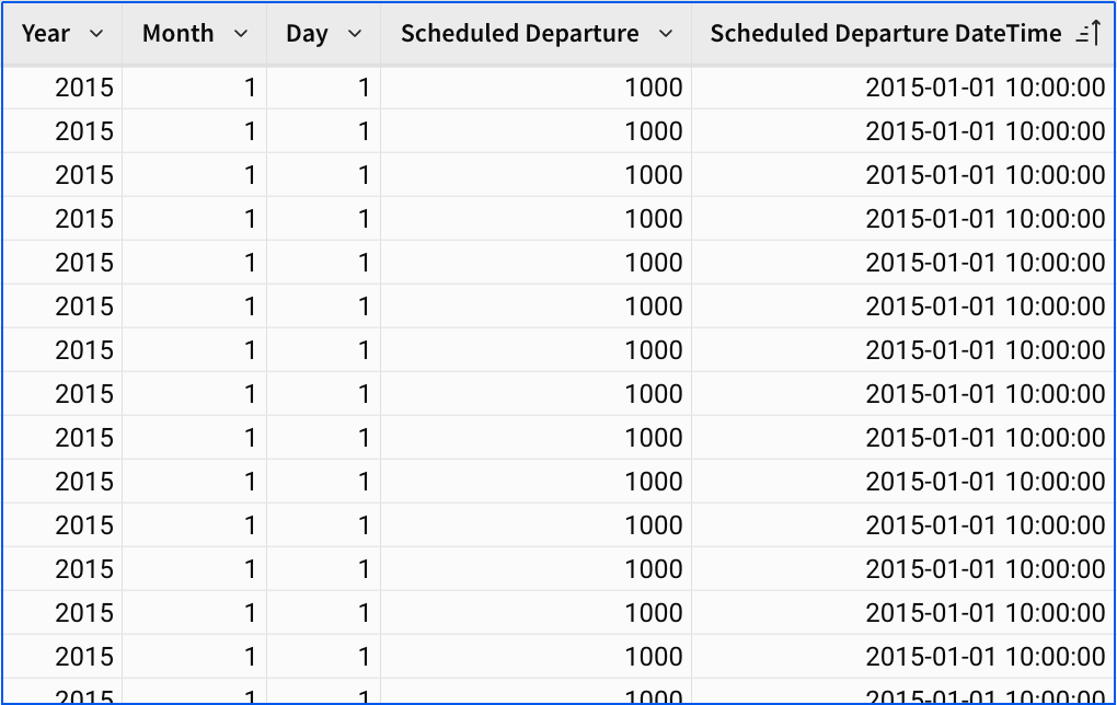
Our end goal for this lesson is to use the formula bar to combine Scheduled Departure with the Year, Month and Day columns to make a single datetime column for ease of use and maintenance. Instead of having four columns to represent a day and time, we want one, like in the example below.

To do this, let’s use Sigma’s MakeDate function. MakeDate requires a year, month, and day as numbers to create a date. Optionally, we can include an hour, minute, and second. Looking at the example provided in Sigma’s documentation, we can see that MakeDate accepts a four-digit year, two-digit month, two-digit day, two-digit hour, and two-digit minute.

We need all five values - year, month, day, hour, and minute - to make a datetime. As we saw earlier when filtering the Scheduled Departure column, our hour and minute values are combined into one column, so let’s separate them.

3. Select the Calc column and rename it Hour of Scheduled Departure.

4. Copy the following formula into the formula bar, then click the green check: Number(Left(Text([Scheduled Departure]), 2))

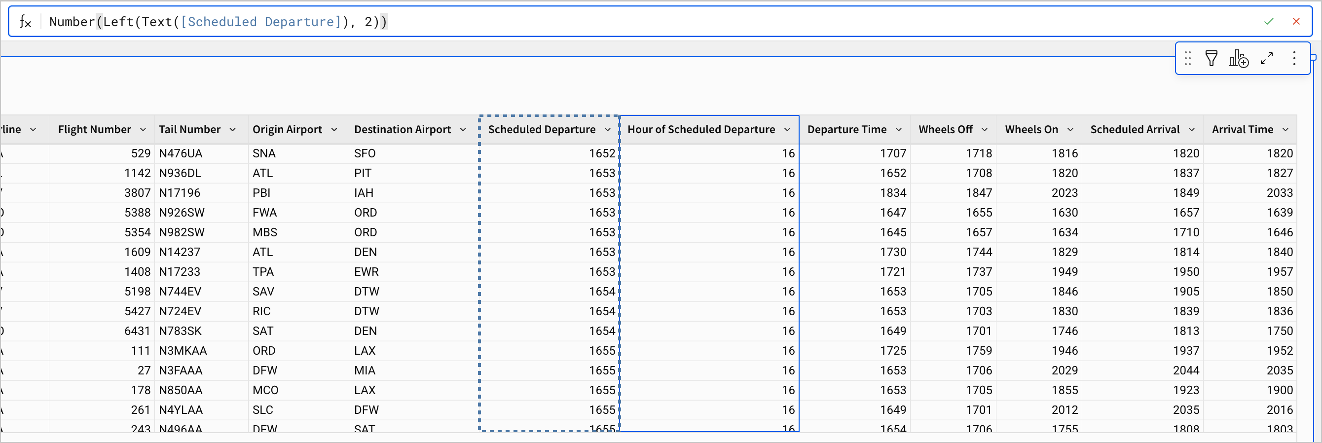
You can see from the result that this takes the two digits that represent the hour from our Scheduled Departure column and returns them as a number. The formula is built around the Left function, which takes the specified number of characters from the left-hand side of a text data entry.

For example, entering Left(“Sigma”, 2) would return “Si”

But if we’d simply entered Left([Scheduled Departure], 2), we’d receive the error message Argument 1 invalid for function Left. Expected text; received number., like below.

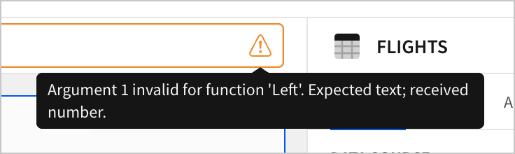
This is because Sigma functions accept and return specific data types. The Left function accepts text data, and returns text data, so we need to change our data types before and after using the Left function. In the provided formula, the first argument for Left is Text([Scheduled Departure]), which uses the Text function to convert the number data in Scheduled Departure to text, so that it is accepted by the Left function. Additionally, we wrapped the whole output in the Number function to return the result as number data.

Let’s repeat this process to extract the minute as a number.

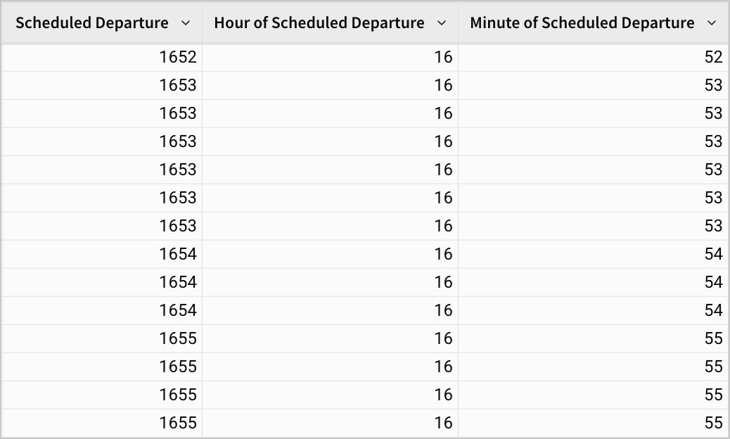
5. Add another new column next to Hour of Scheduled Departure, and name it Minute of Scheduled Departure. Use the following formula: Number(Right(Text([Scheduled Departure]), 2))

This creates a number column with our minute data. It works just like the formula for the hour, except it takes the two right-hand digits, which represent the minute.

With hour and minute separated into their own columns, let’s try using MakeDate.

6. Create a new column next to Scheduled Departure. Name it Scheduled Departure DateTime, and enter the following formula: MakeDate([Year], [Month], [Day], [Hour of Scheduled Departure], [Minute of Scheduled Departure])

You should see a result like the below:

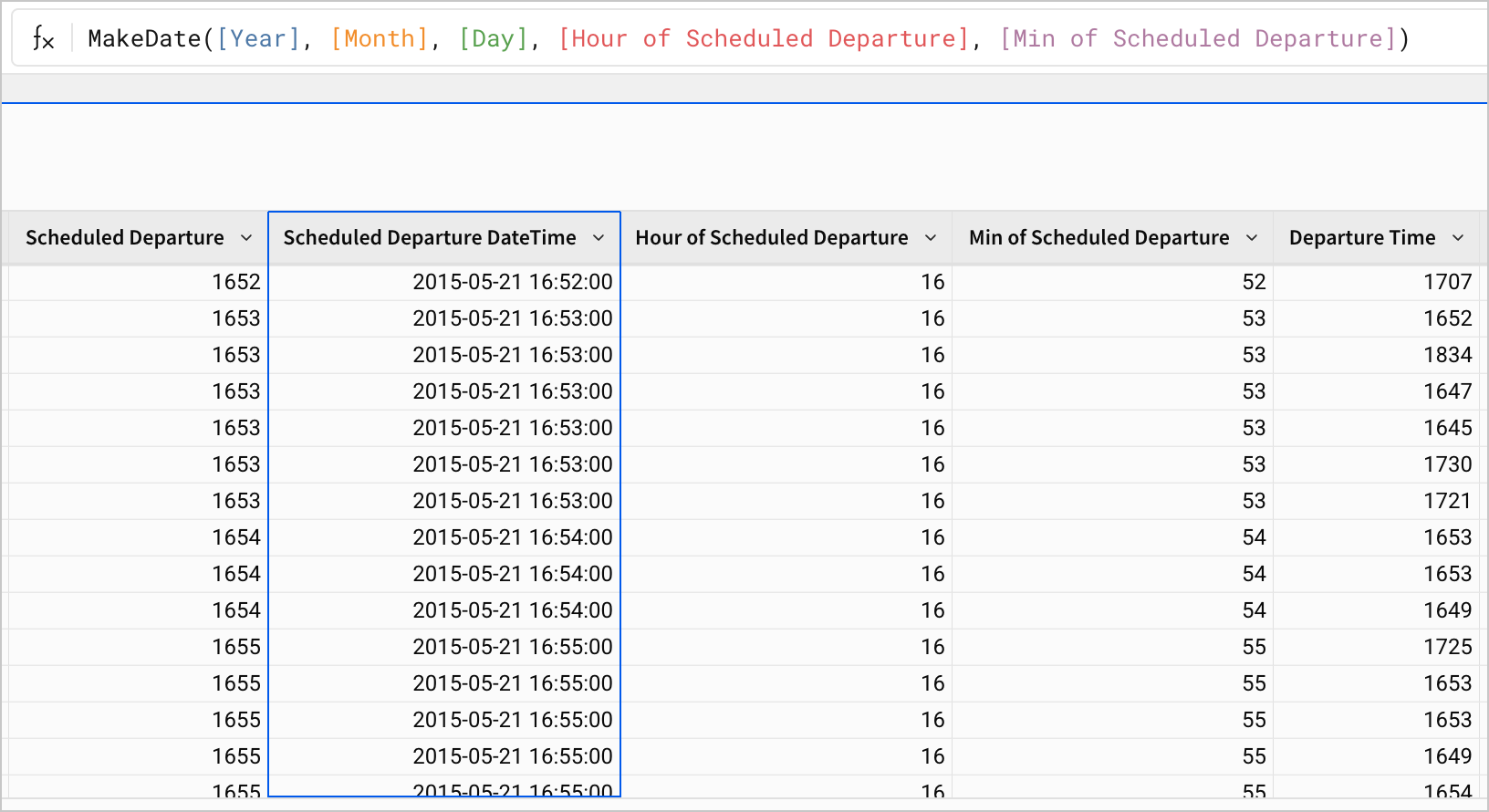
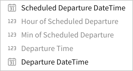
If you look at this new column under the column list in the editor panel, you’ll see that the icon indicates it is date data.

7. Click Publish to save your work to the published version.

Repeating our transformations

Each data type provides its own shortcuts that we can use when working with that it. For example, the automatic selection of the sum aggregate when creating a new summary, or of the number range filter type when filtering Scheduled Departure, both apply because the column has the number data type.

By building a column with the date data type, we’ve given ourselves access to the functionality that comes with it, like automatic filtering by date range, automatic time axes on charts, and more. That functionality is used in later sections of this tutorial, particularly in lessons 4 through 8.

But, we’ve only done this transformation for one of the several timestamps in our dataset. We still have Departure Time, Wheels Off, Wheels On, Scheduled Arrival, and Arrival Time stored as number data. Before we conclude, let’s transform these as well, and then organize our table.

To start, let’s make these transformations easier. When first transforming the Scheduled Departure data, we made separate columns for hour and minute data, which held the outputs of our substring formulas. We then passed those new columns into the MakeDate function. This workflow was helpful as we familiarized ourselves with data types and formulas, but we don’t need to repeat all of these steps for each time column.

Instead, we could choose to handle all our transformations inside one formula.

1. Create a new column, and name it Departure DateTime.

📘

Departure Time is different from Scheduled Departure. Departure Time is the time the plane actually departed, rather than the time it was scheduled to depart.

2. Copy the following formula into the formula bar for that column: MakeDate([Year], [Month], [Day], Number(Left(Text([Departure Time]), 2)), Number(Right(Text([Departure Time]), 2)))

This creates a column of date data for the Departure Time:

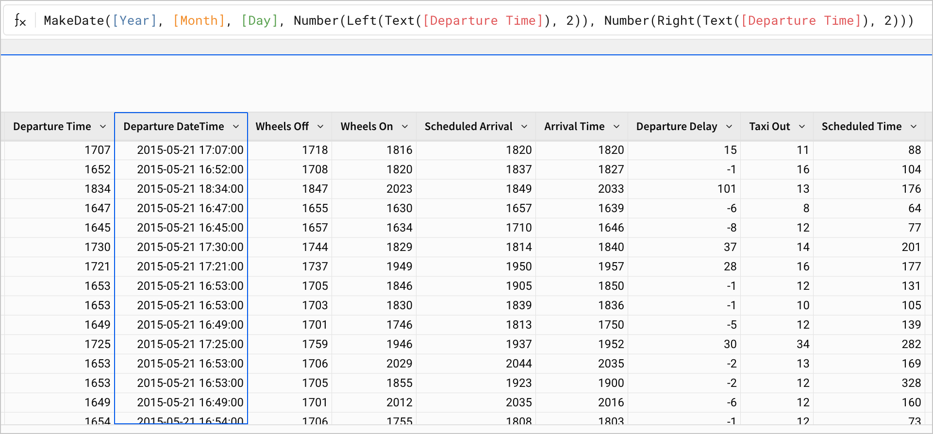
We used our formulas for extracting the hour and minute as arguments to the MakeDate function, rather than making additional columns and passing those values to MakeDate. We can repeat this to convert all timestamp columns into dates.

3. Create new columns for Wheels Off DateTime, Wheels On DateTime, Scheduled Arrival DateTime, and Arrival DateTime.

4. In the formula bar for each new column, use the formula above as an outline to convert these number columns into dates by replacing the column references for each target column. For example, the formula for Wheels Off DateTime looks like this: MakeDate([Year], [Month], [Day], Number(Left(Text([Wheels Off]), 2)), Number(Right(Text([Wheels Off]), 2)))

When you’re done, your table might look something like this:

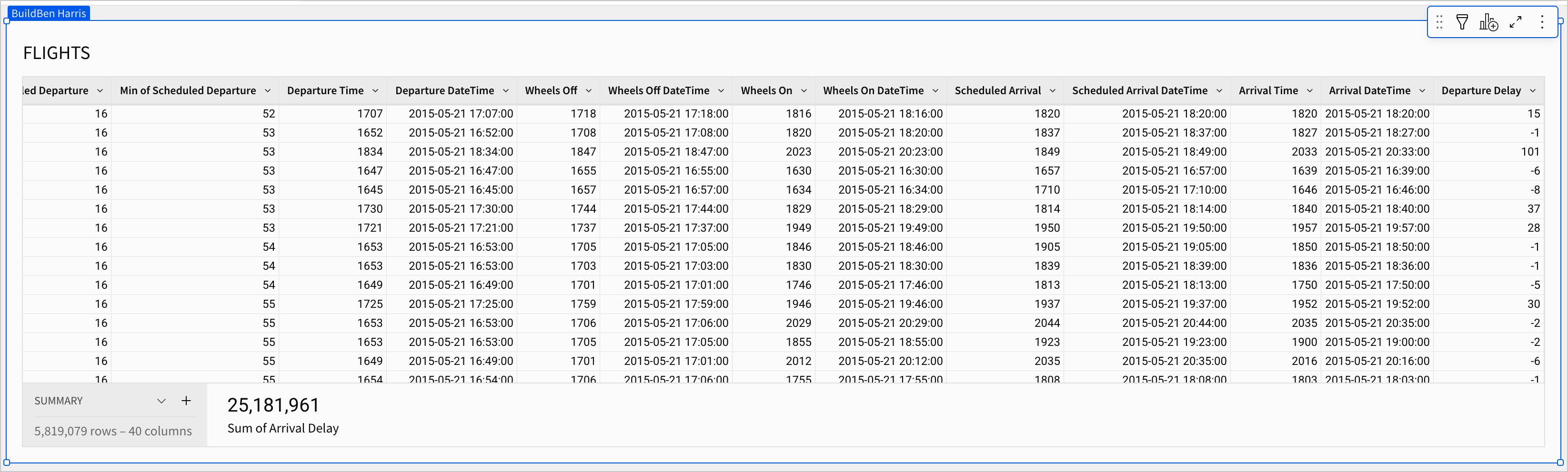
5. Click Publish to save your work to the published version.

Organization

We now have access to all of our timestamps as dates, but our table’s legibility and organization have suffered. We have many duplicate columns, and the width of the table makes it difficult to read.

To solve this, let’s organize our columns again and hide duplicates.

1. Scroll over to the columns Hour of Scheduled Departure, Min of Scheduled Departure, and Scheduled Departure.

2. Hold shift on your keyboard, and click on Hour of Scheduled Departure, then Scheduled Departure to select all three columns. Open the column menu for any of them, and select Hide 3 columns.

The columns are now hidden. They don’t appear in the table to you, and they don’t appear to end users. However, you can still see them grayed out in the editor panel.

They also still appear in calculations in other columns. This is why we’ve chosen to hide them instead of deleting them. All of our formulas from previous steps still function when referencing a hidden column.

3. Hide the following columns:

• Year
• Month
• Day
• Scheduled Departure
• Wheels Off
• Wheels On
• Scheduled Arrival
• Arrival Time

Your table summary now shows 29 columns.

4. Finally, drag and drop the new date columns to the left of the table, so that each record begins with the various timestamps associated with the flight.

5. Click Publish to save your work to the published version.

Conclusion

At the end of lesson two, we’ve familiarized ourselves with our dataset and transformed it for future use. To do so, we learned about:

• Table summaries
• Sorting
• Filtering
• Data types in Sigma
• Formulas in Sigma
• Hiding and organizing fields
• And more!