Format pivot table totals

In addition to customizing all cells in a table or pivot table by applying table styles, you can format pivot table totals separately from the other values in a pivot table:

Apply unique formats to subtotals and grand totals in a pivot table, described in this document.
Change the number format and appearance of totals rows and columns using the toolbar. See Format column and totals data.
Apply conditional formatting to subtotals and grand totals. See Apply conditional formatting.

To show or hide subtotals and grand totals, see Pivot table totals and subtotals.

This document describes the format options for pivot table totals and explains how to customize the display of rows and columns containing subtotals and grant totals.

User requirements

The ability to format pivot table totals requires the following:

You must be assigned an account type with the Explore workbooks or Create, edit, and publish workbooks permission enabled.
You must be the workbook owner or be granted Can explore or Can edit workbook permission.

Pivot table totals format options

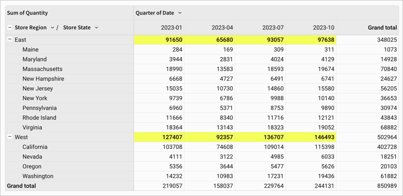
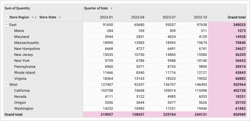
Subtotals

The Subtotals tools allow you to customize the font weight, font color, and background color of subtotal rows and columns.

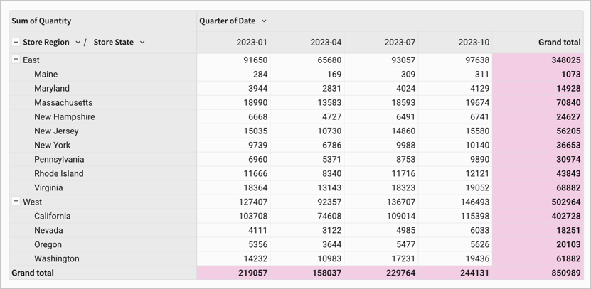
Grand totals

The Grand totals tools allow you to customize the font weight, font color, and background color of the grand totals row and column.

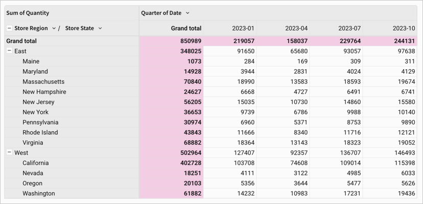
Position

The Position setting allows you to move grand totals to the first or last column and row.

First	Last

Format pivot table totals

Open a workbook in Explore or Edit mode.
Select the pivot table you want to format.
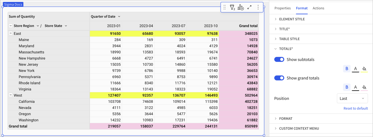
Select Element format in the side navigation, then click the Totals header to expand the section.
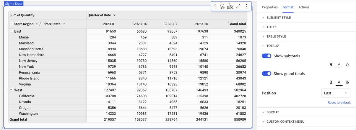
Use the Subtotals and Grand totals tools to customize font weight, font color, and background color, and select an option in the Position dropdown to control the position of the grand total row and column.