Working with pivot tables
With Sigma, you can create a pivot table to group and summarize your data in a particular way. Use a pivot table to present your data in two dimensions, automatically summarize your data based on groups, and view your data in various hierarchies.
You can group columns in a table to approximate some functionality in pivot tables, such as aggregating data for specific groups. See Create and manage tables.
Requirements
- To create or edit a data element, you must have Can edit access to the individual workbook.
- Some exploratory actions are also supported with Can explore access.
For more details, see Folder and document permissions.
Create a pivot table
You can create a pivot table from an existing data element, or from the Add element bar by selecting Data > Pivot table. For more details, see Create a data element.
A pivot table does not display data until you define the data source columns to use as pivot rows and/or pivot columns. Configure the following properties in the Properties tab of the editor panel:
-
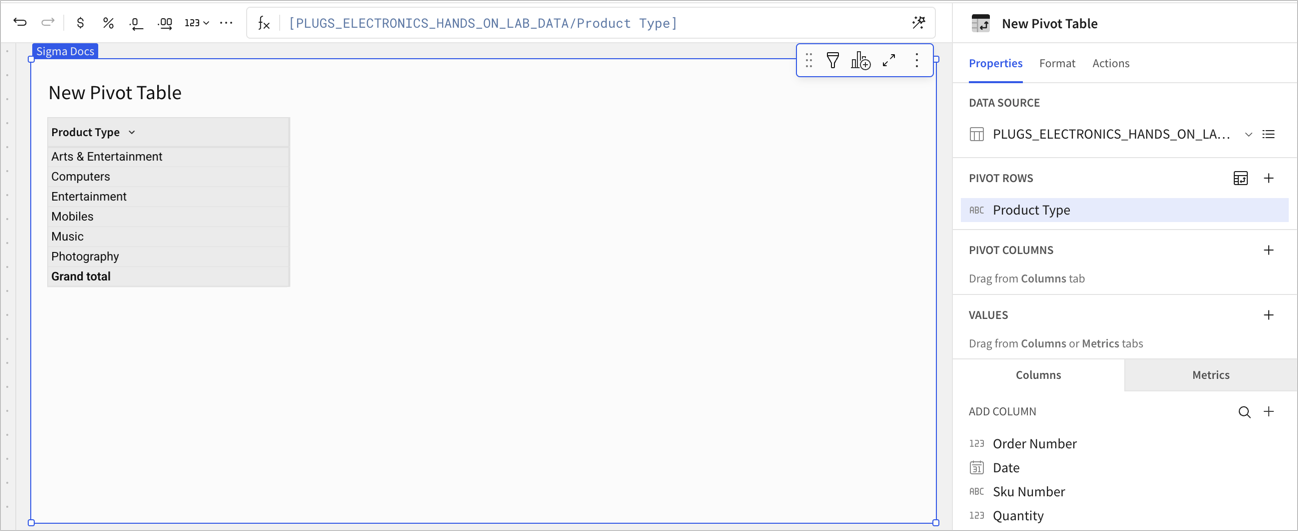
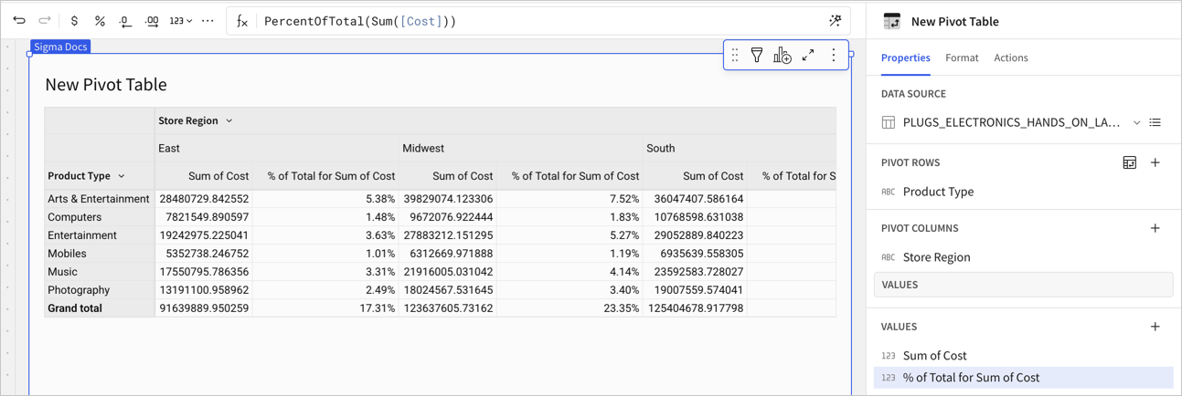
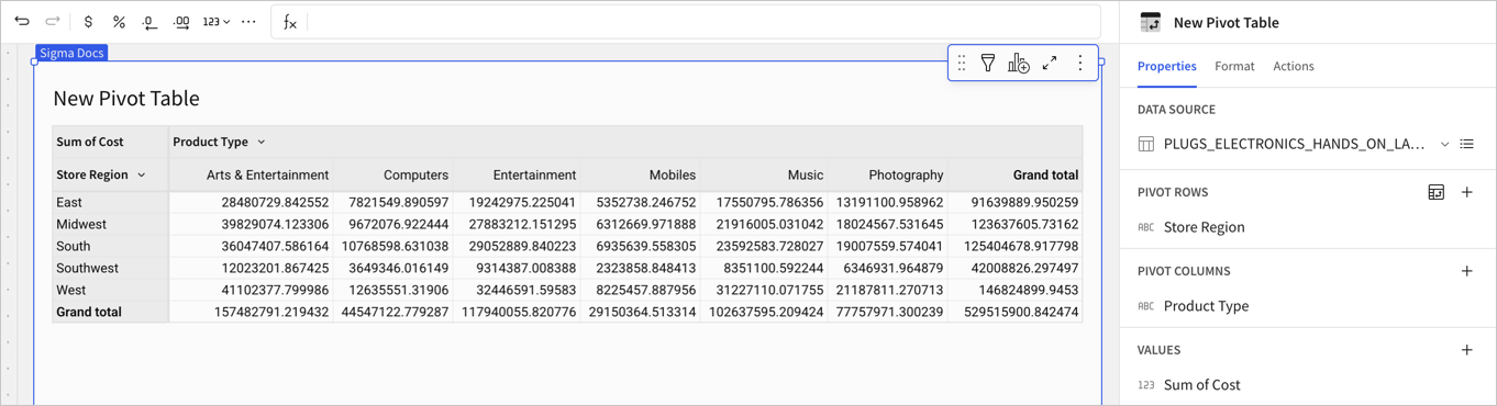
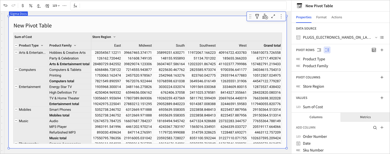
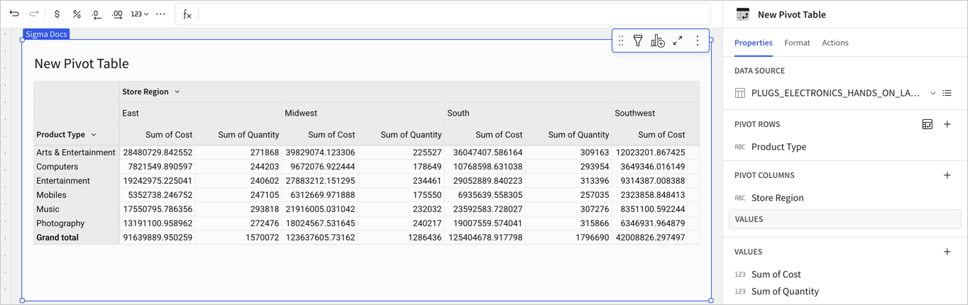
Pivot rows: Select one or more columns from your table to appear as rows in the pivot table. For example, to summarize total cost for product type, add the product type column as a Pivot row.
-
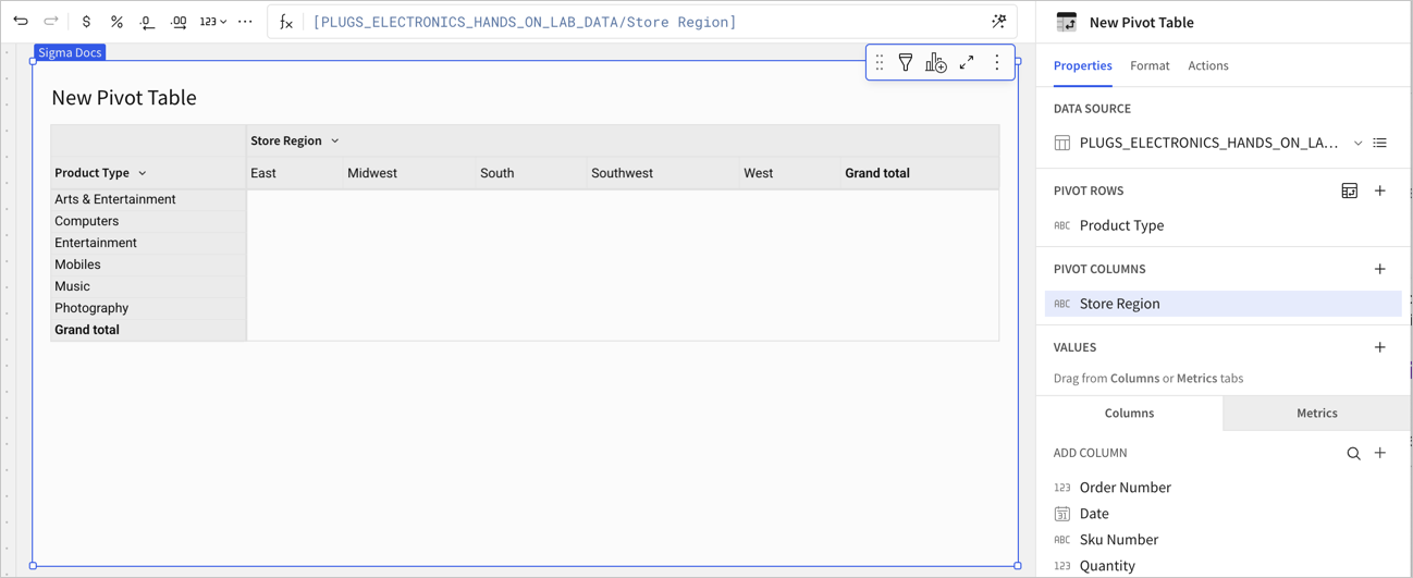
Pivot columns: Optional if you define one or more pivot rows. Select one or more columns to split the values in each row. For example, to summarize the total cost for each product type in each store region, add the store region column as a pivot column.
-
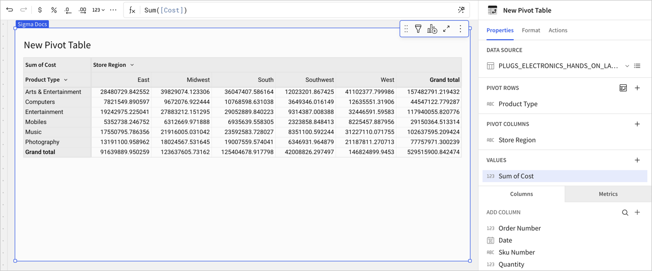
Values: Select one or more columns to display the values for each pivot row and column. Columns added to Values are aggregated by default and the type of aggregation used depends on the data type of the original column. For example, add the cost column as a value, and leave the default aggregation of Sum, or adjust it by rounding. See Change the aggregation of values.
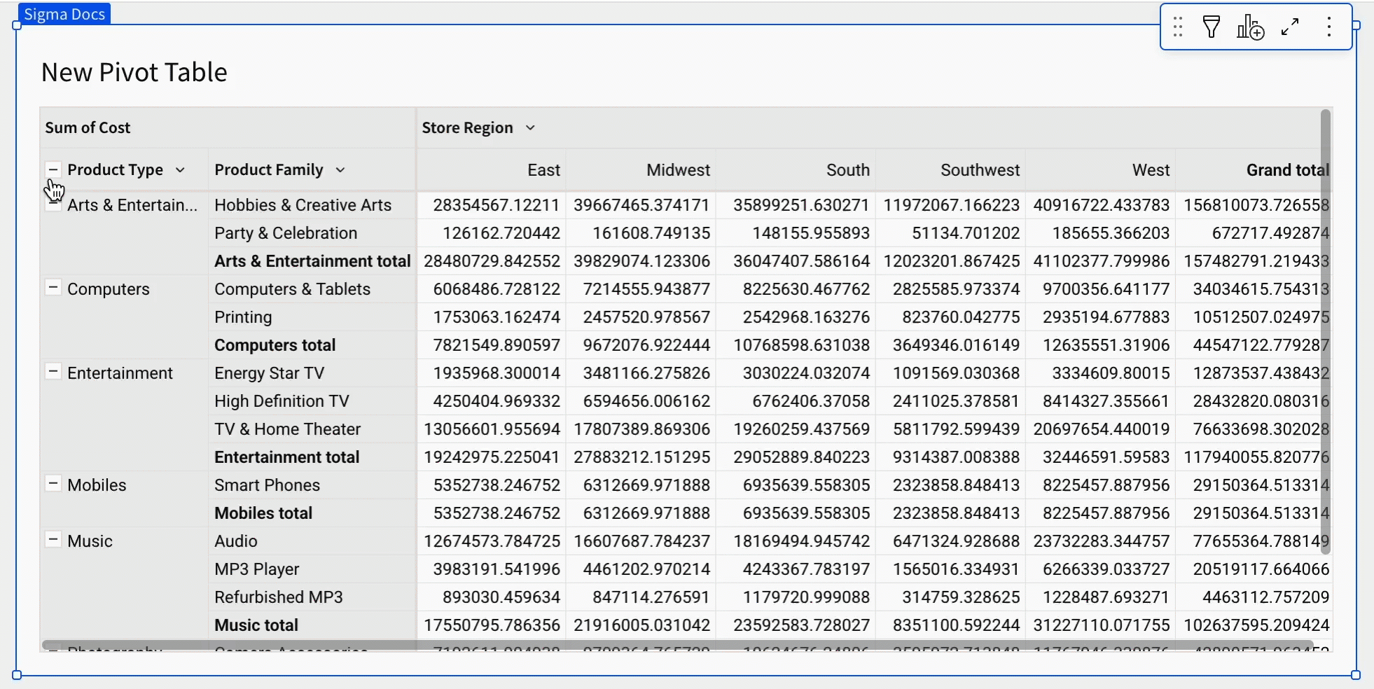
Once your table has been created, you are able to select all cells, rows, columns, and headers in pivot tables, including fixed or empty headers.
To select a range of cells in your table, select the first cell in your range, then press the Shift key on your keyboard and select another cell. If you select multiple cells of the same data type, the aggregate of the cells is displayed at the bottom of the table. The aggregation methods available depend on the selected data type, and can be changed by selecting the ![]() down arrow.
down arrow.
Pivot table formatting and customization options
You can customize the formatting and presentation of a pivot table in many ways. To show or hide totals in a pivot table, see Pivot table totals and subtotals.
Before you start: This task requires editing elements. You can edit an element by customizing or editing a workbook.
- In the editor panel, select the Format tab.
- Click a format category to view and edit its settings.
The following format categories are available for pivot tables:
- Element Style: See Customize element background and styles.
- Title: See Customize element title.
- Table style: See Format and customize a table.
- Totals: See Format pivot table totals.
- Format: See Specify empty cell display value and Repeat row labels.
You can also format pivot table columns. See Format pivot table columns.
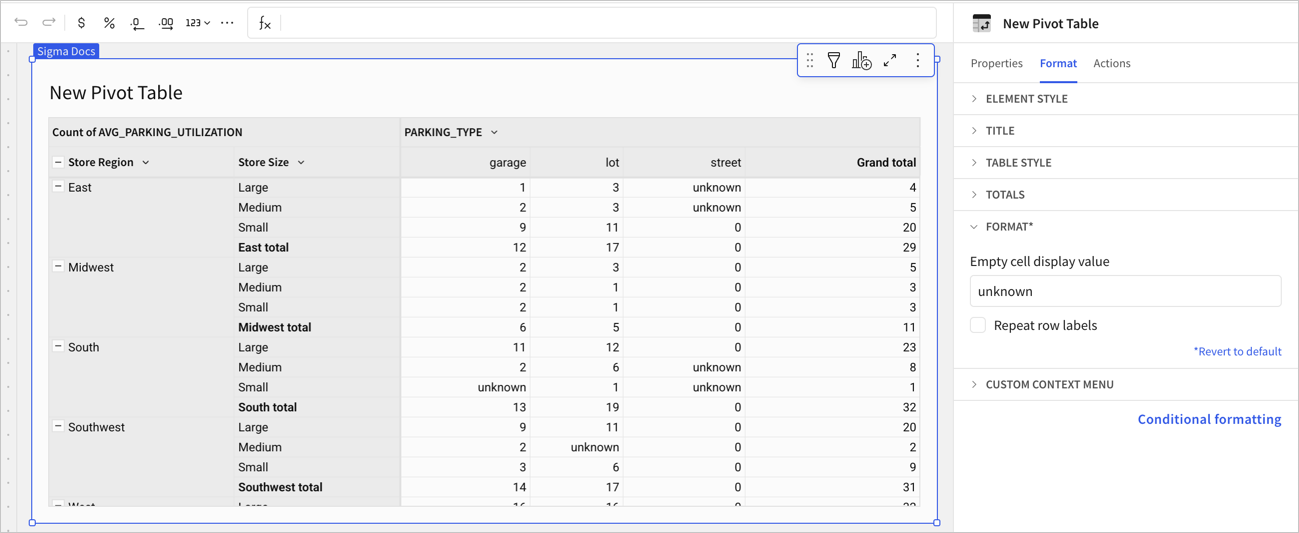
Empty cell display value
If you have empty values in a pivot table, you can specify a value to fill the empty cells.
- Open a workbook for customizing or editing.
- Select a pivot table element, then in the editor panel, select the Format tab.
- Click Format.
- For Empty cell display value, enter a value.
Repeat row labels
If you have multiple pivot rows defined, and you choose to display the pivot row groupings as separate columns, you can repeat the row labels:
- Open a workbook for customizing or editing.
- Select a pivot table element, then in the editor panel, select the Format tab.
- Click Format.
- For Repeat row labels, select the checkbox.
Format pivot table columns
The following column formatting options are available:
- Alignment
- Font color
- Background color
- Conditional formatting
Apply basic visual column formatting
To change the alignment, font color, or background color of values in a column:
- Select the column or cell that you want to format.
The fixed headers in the table can be used to quickly apply formatting changes:
- If you want to format all the cells in your table and you only have one Value set, select the fixed value header in the upper left corner of the table, then configure your formatting changes. Your changes will be applied to all cells.
- To format all row/column header cells, select the fixed row/column header and apply your changes. If you have multiple pivot rows in stepped layout or multiple pivot columns configured, your changes will only be applied to header cells of the first row/column.
- To set the background color, select
 Background color in the formula bar.
 - To set the font color, select
 Text color in the formula bar.
 - To set the alignment of the data, select
 Alignment in the formula bar.
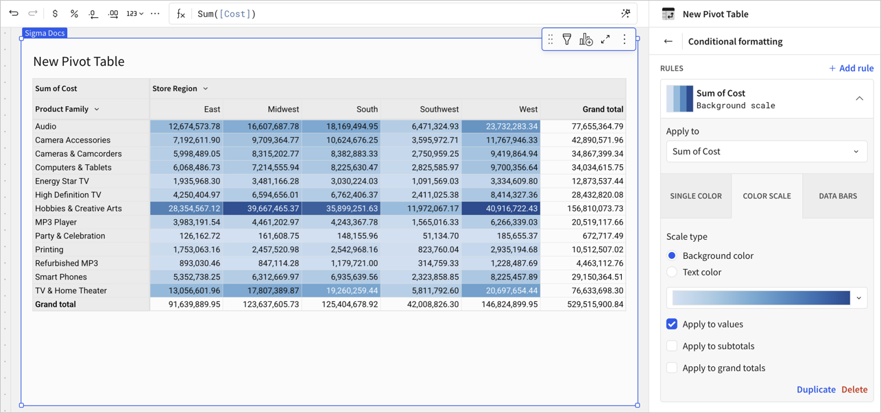
Apply conditional formatting
You can apply conditional formatting to the columns, rows, and values in a pivot table. Use conditional formatting to show different background colors for different values, highlight discrepancies in data with a background or font scale, or display data bars to quickly visualize outlier values.
Conditional formatting takes precedence over toolbar column formatting options.
Before you start: This task requires editing elements. You can edit an element while customizing or editing a workbook.
-
Open a workbook for customizing or editing.
-
Select a pivot table element, then in the editor panel, select the Format tab.
-
Click Conditional formatting.
-
Click + Add rule.
-
Customize the rule:
- Choose a column to apply the formatting to
- Choose whether to use a single color, color scale, or add data bars to cells
- Select checkboxes to apply the formatting to values, subtotals, or grand totals.
Change data presentation in a pivot table
While most complex data transformations for a pivot table should occur in the flattened source table, you can manipulate the presentation of data in a pivot table in several ways:
- Change the aggregation of values
- Add a calculated column to a pivot table
- Swap pivot columns and rows
- Display multiple pivot rows as separate columns
- Collapse grouped rows and columns
- Define values hierarchy in a pivot table
- Hide or show fixed pivot table headers
- Aggregate totals across higher grouping levels
These tasks requires editing elements. You can edit an element while customizing or editing a workbook.
Change the aggregation of values
When you add a data column to a pivot table’s Values field, the values are automatically aggregated according to the data type. Numeric columns are aggregated by Sum, while text and date columns are aggregated by Count.
To change a column’s aggregation:
- In the editor panel, hover over the column, and click the down arrow (
 ).
The column menu opens.
).
The column menu opens. - From the Set aggregate submenu, select a new aggregate. For example, choose one of Sum, Avg, Median, Percentile, Min, Max, First, Last, Count, CountDistinct, or more advanced calculations like percent of total.
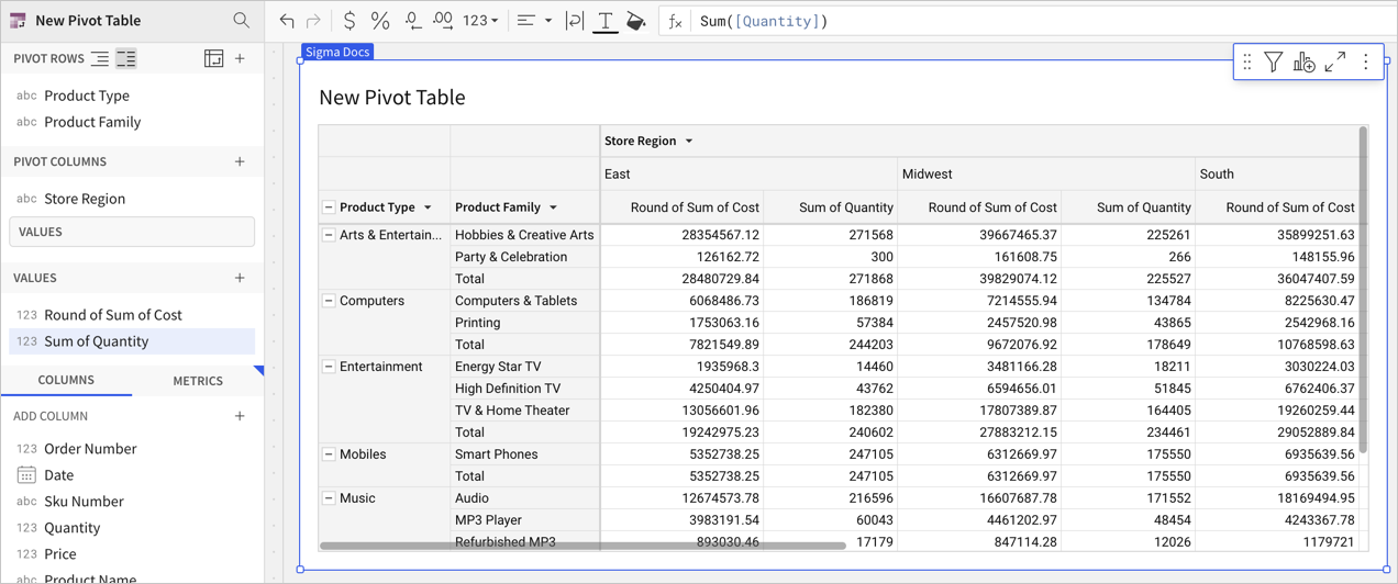
Add a calculated column to a pivot table
Add a calculated column to a pivot table to perform a calculation that repeats across the pivot, such as a percentage of total or a period-over-period analysis.
-
Select the pivot table element.
-
In the Values section, select + > Add new column. A new column titled Calc appears and the focus changes to the formula bar.
-
Enter a formula for the calculated column, then press Enter on your keyboard or select the checkmark to save. The column is automatically renamed after the formula.
For guidance working with pivot table totals in calculated columns, see Pivot table totals and subtotals.
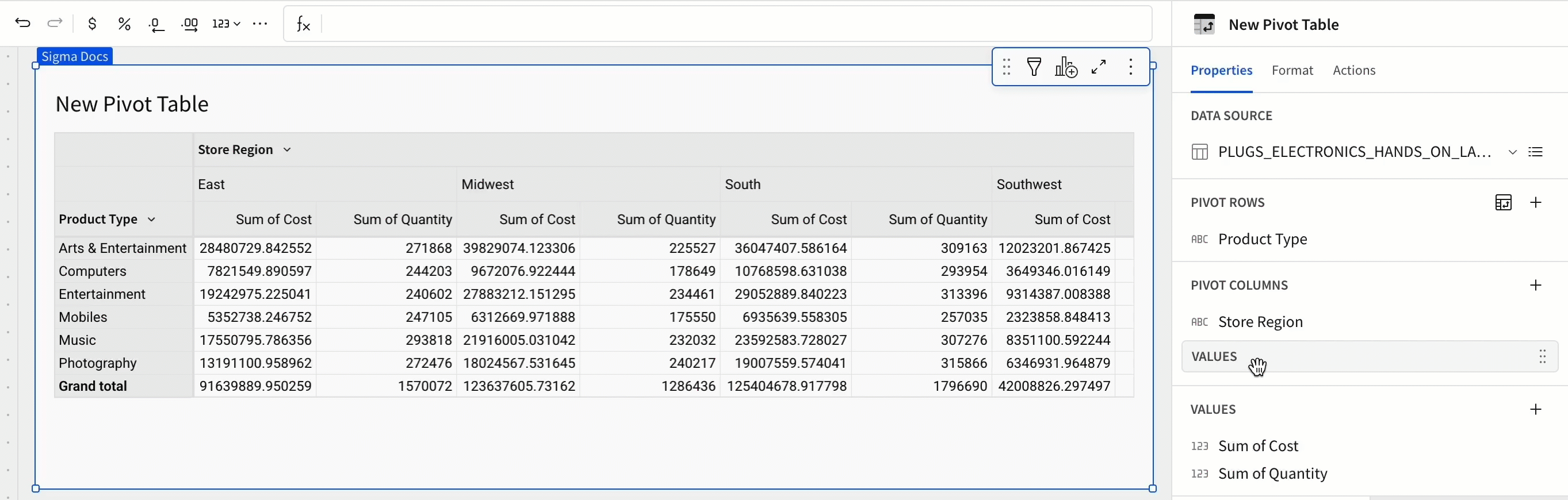
Swap pivot columns and rows
You can change the layout of your pivot table and swap rows with columns:
-
Select the pivot table element.
-
In the editor panel, next to the Pivot rows header, click
 Swap rows with columns.
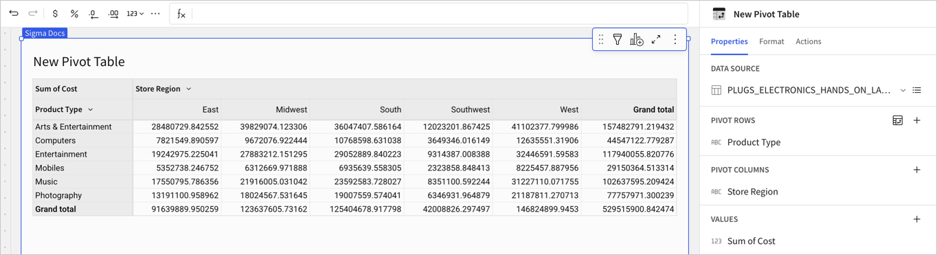
Pivot table rows are swapped with columns.
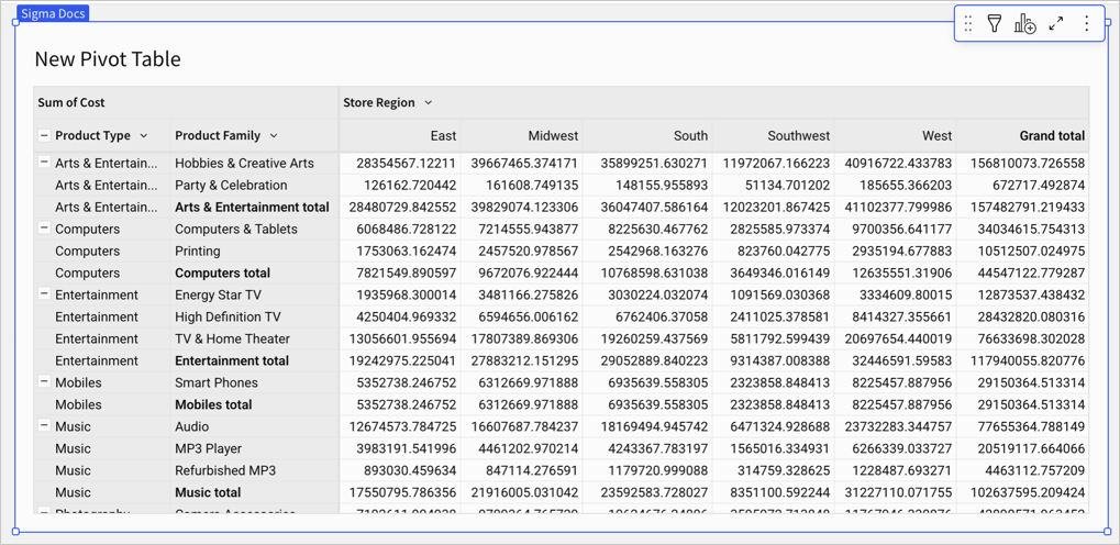
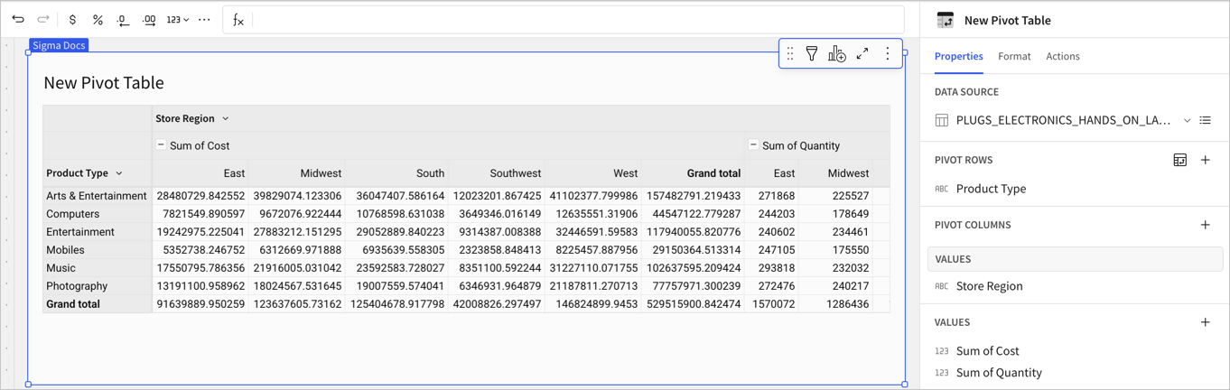
Display multiple pivot rows as separate columns
When you have multiple pivot rows, you can choose to display the data combined in one column, or as separate columns.
After adding a second data column as a pivot row, select ![]() Display as separate columns. To change the display back, select
Display as separate columns. To change the display back, select ![]() Display as a single column:
Display as a single column:
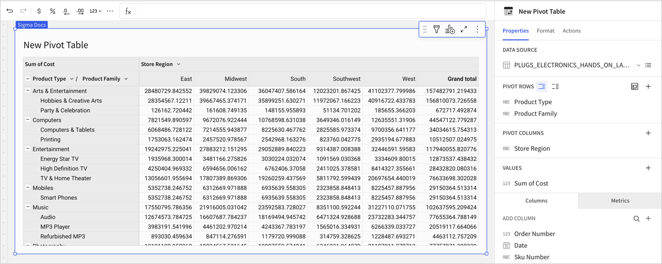
Collapse grouped rows and columns
If your pivot table has at least two data columns added as Pivot rows or Pivot columns, you can expand and collapse the rows and columns. To do so, click + or - next to the value of a pivot table row, column, or cell header.
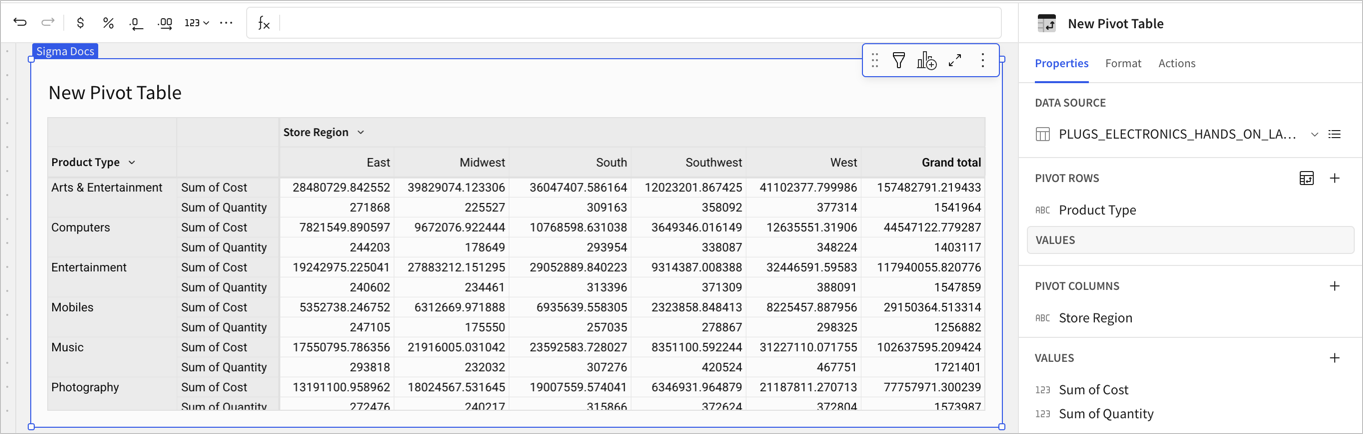
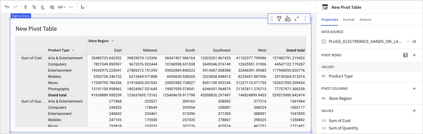
Define values hierarchy in a pivot table
If you have multiple values in your pivot table, you can define the hierarchy and groupings of data columns, values, and rows to reflect the data summaries that you want to display.
To structure the hierarchy of values in your pivot table:
-
Select the pivot table element.
-
Add at least two columns as Values.
A box labeled Values appears under Pivot columns:
-
To change the default hierarchy, drag and drop the Values box to another position under Pivot columns or to Pivot rows.
The data presentation changes based on the location of the values:
Hide or show fixed pivot table headers
You can hide or show fixed row and column headers in pivot tables. This can be useful to create additional space within a table for summary statistics, or reduce the visual space a table occupies within a workbook.
To hide or show fixed pivot table headers:
-
Select your desired table. From the editor panel, select the Format tab.
-
Expand the Table components section.
-
Turn the Show column headers toggle and Show row headers toggle on or off to show/hide headers.
Hiding fixed column headers will also hide fixed value headers (the header in the upper left corner of your pivot table if you only have one Values column specified). If you have multiple Values columns, hiding column headers will not affect the appearance of value headers.
-
Select Reset to default to return to the default setting (show all row and column headers).
Exporting workbooks with fixed pivot headers hidden is only supported for PDF and PNG exports. Changes to table formatting made with this feature are not reflected in other export destinations.
Aggregate totals across higher grouping levels
When you display subtotals in your pivot table, you can change whether the row subtotals are aggregated and displayed for the immediate parent pivot rows or also displayed at higher grouping levels. By default, totals are aggregated only at the immediate parent row level.
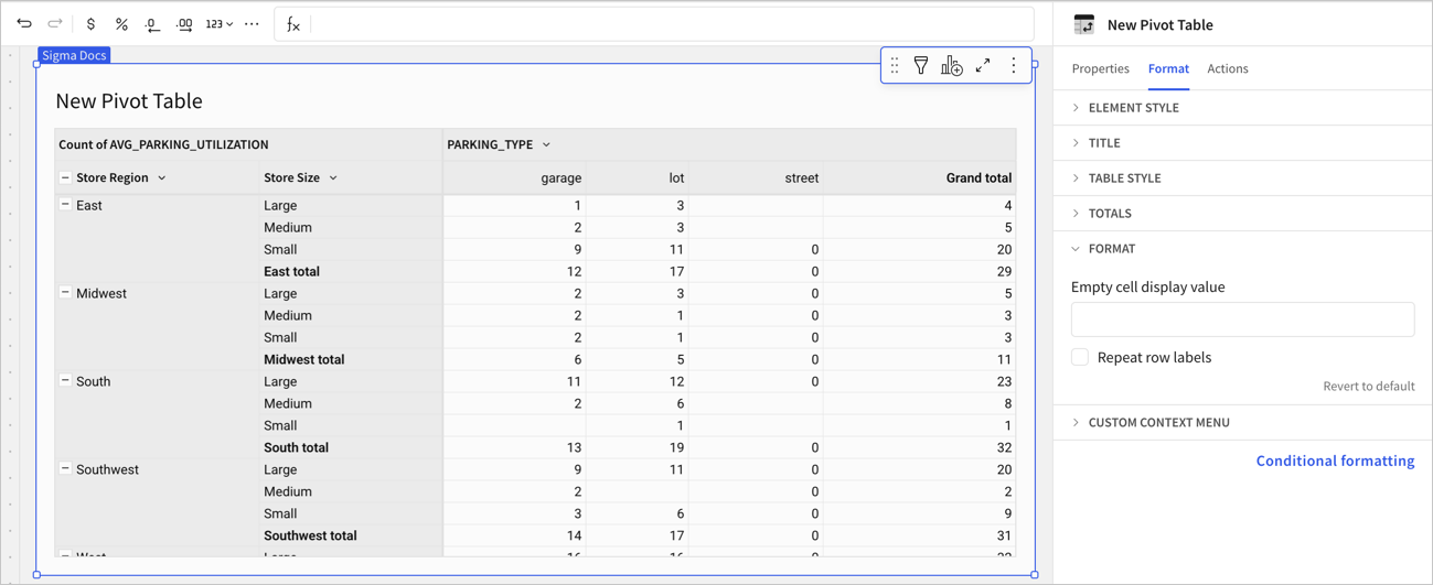
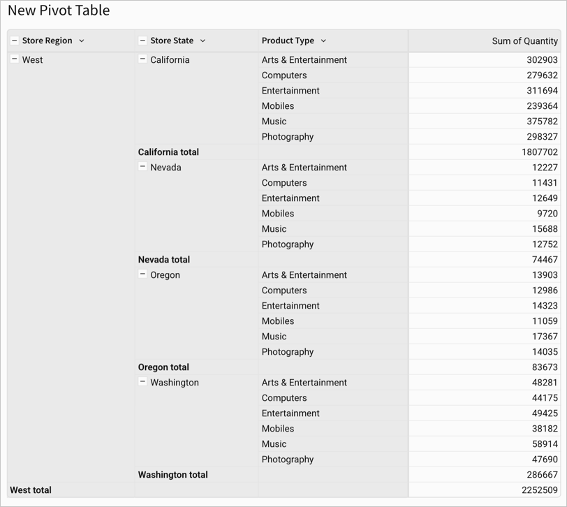
For example, in a pivot table created using the PLUGS_ELECTRONICS_HANDS_ON_LAB_DATA data source with the following pivot rows:
- Store Region
- Store State
- Product Type
And a pivot values column of Quantity, the subtotals of Product Type are shown for each Store State:
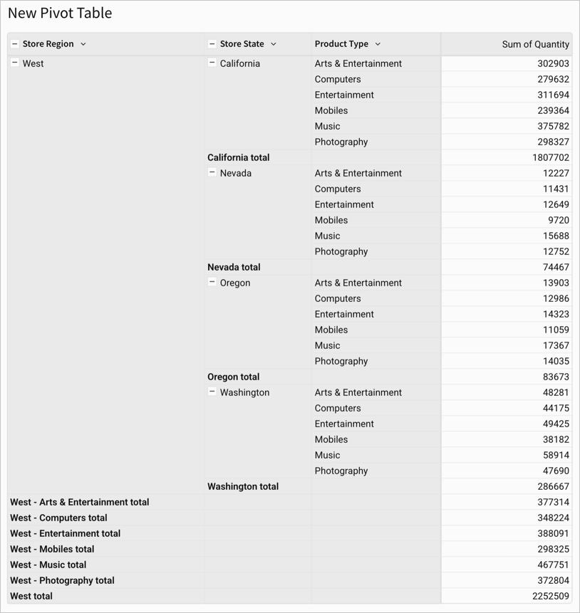
To instead see the Sum of Quantity for each Product Type in each Store Region, you can do the following:
-
Right-click on one of the Product Type rows or select the down arrow (
) for the Product Type column to open the column details menu, then select Totals of Product Type. -
For Show values aggregated at, select Every parent row.
Your pivot table updates to display the subtotal for each Product Type at the region level and the state level:
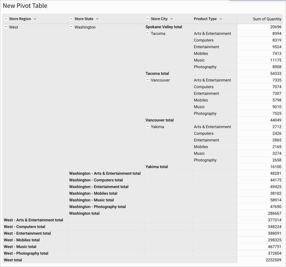
Aggregating pivot row totals at every parent level persists even if new parent levels are added. For example, if you add the Store City column to the pivot table, the Product Type totals are visible at the Store State and Store Region levels:
Maximize a pivot table to view the flattened table
When viewing, customizing, or editing a workbook, all data elements are minimized by default to display multiple elements in the canvas. You can maximize any data element to focus on its details and explore the underlying data.
Select ![]() Maximize element, or press the space bar on your keyboard with an element selected, to view the underlying data.
Maximize element, or press the space bar on your keyboard with an element selected, to view the underlying data.
When you maximize a pivot table, it expands to the full width of the workbook page and displays the underlying flattened data table. You can use this view to explore the grouping levels of the pivot table. Because the element and underlying data are inherently linked, changes applied to one are automatically reflected in the other.
You can only make changes to the underlying data of a data element while customizing or editing a document.
For more details, see View underlying data.