MovingVariance

The MovingVariance function calculates the statistical variance of a column in a moving window.

Syntax

MovingVariance(\[column\], above, below)

Function Arguments:

• [column] (required) - The column of numbers to calculate the variance.
• above (required) - The first row to include, counting backwards from the current row.
• below (optional) - The last row to include, counting forward from the current row. Defaults to 0 (current row will be the last row included).

📘

When using this function without a sort enforced, there can be unexpected results. In order to ensure that the values are stable, verify that there is a sorted column within the table.

Example

A table contains the daily close price of a stock in 2016. Variance can be used to show the volatility of a stock, where a higher variance indicates higher risk. We can use the MovingVariance function to identify the change in variance in different moving windows.

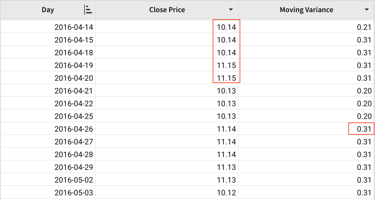
MovingVariance(\[Close Price\], 4)

With [Close Price] as the column argument and 4 as the above argument, the variance will be calculated for each week along with the four previous weeks. Since the below argument was not specified, it defaults to 0.  

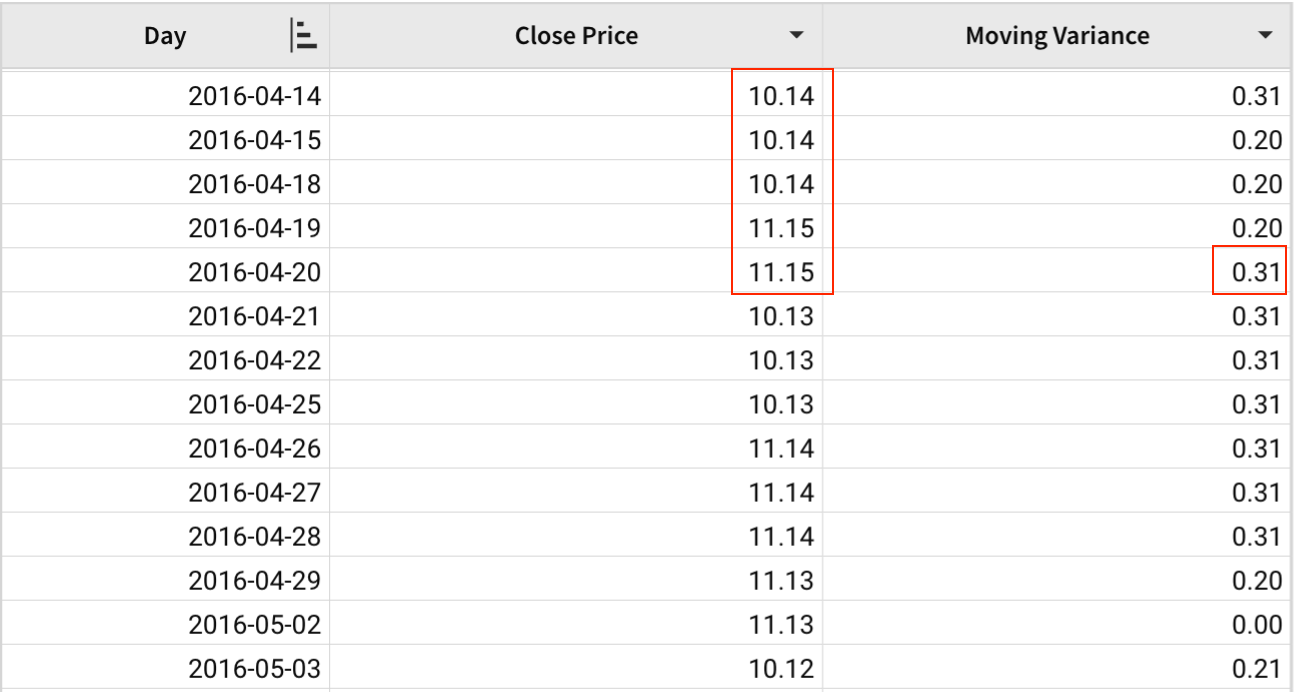
MovingVariance(\[Close Price\], 0, 4)

Here, the above argument is 0, so there will not be any previous weeks included in the window. The below average is 4, so the variance will be computed for each week along with the next 4 weeks.

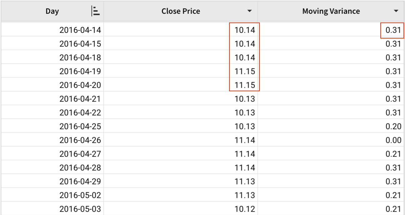
MovingVariance(\[Close Price\], 2, 2)

Here, the above argument is 2, so the previous two weeks will be included in the window. In addition, the below argument is 2, so the following two weeks will be included as well.

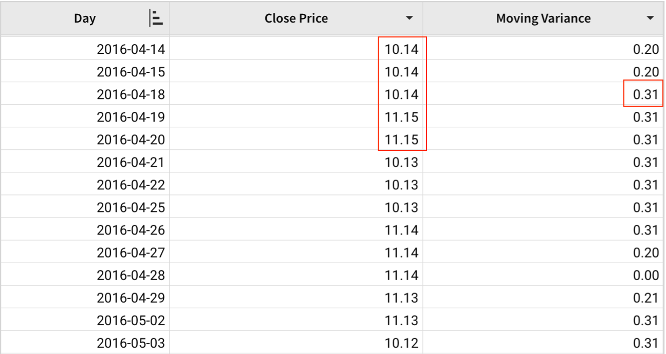
MovingVariance(\[Close Price\], 8, -4)

Here is an example where the below parameter is negative. The below parameter can be negative as long as the value is less than that of the above parameter. In this example, each window begins 8 weeks before the current week and ends 4 weeks before the current week, inclusive.