> For clean Markdown of any page, append .md to the page URL.
> For a complete documentation index, see https://help.sigmacomputing.com/llms.txt.
> For AI client integration (Claude Code, Cursor, etc.), connect to the MCP server at https://help.sigmacomputing.com/_mcp/server.
# Pivot table totals and subtotals
Grouped tables and pivot tables calculate totals and subtotals. If your pivot table contains aggregated values, such as the sum or count of a value, totals are shown by default.
You can hide, manage, customize, and perform additional calculations with totals and subtotals in a grouped table or pivot table.
* To hide totals, see [Show and hide totals in a pivot table](#show-and-hide-totals-in-a-pivot-table) or [Show totals in a grouped table](/docs/create-and-manage-tables#show-totals-in-a-grouped-table)
* To customize the formula used to calculate totals, see [Customize totals and subtotals](#customize-totals-and-subtotals)
* To format totals, such as by highlighting totals or changing the font color, see [Format pivot table totals](/docs/format-pivot-table-totals).
For more details about tables, see [Create and manage tables](/docs/create-and-manage-tables).
For more details about pivot tables, see [Working with pivot tables](/docs/working-with-pivot-tables).
## Definitions and key concepts
Grand totals are calculated if a pivot table contains values, or a grouping in a table contains calculations. Subtotals are calculated if a pivot table contains values and has more than one column added as a pivot row or pivot column, or a table contains multiple groupings with calculations.
By default, totals are calculated using the same formula as the corresponding value in a pivot table or table grouping, but applied to a higher-level grouping of the data. If you want to change the formula used to calculate totals, see [Customize totals and subtotals](#customize-totals-and-subtotals).
Grand total calculations are performed against the entire table or pivot table, and subtotal calculations are performed against each grouping of the data:
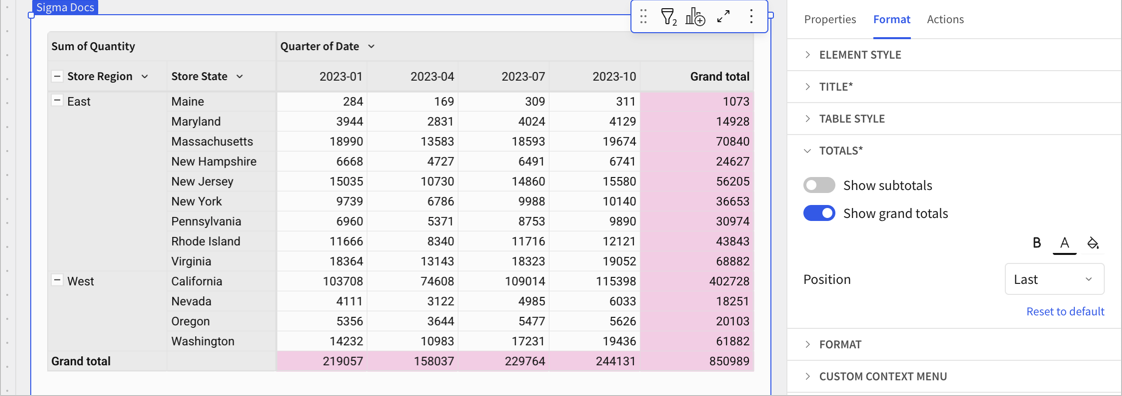
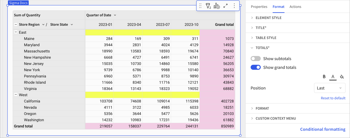
* **Grand total**: The aggregated calculation of **all** values for a pivot row, pivot column, or grouping calculations. In the example screenshot, grand totals are highlighted in pink.
* **Subtotal**: The aggregated calculation of values in **a group** of pivot rows, pivot columns, or a given table grouping. In the example screenshot, subtotals are highlighted in yellow.
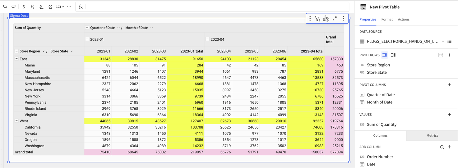
In a grouped table, only the grand totals for each grouping are available for use in formulas. For a pivot table, depending on how many pivot rows, columns, or values exist, other calculated totals might be available to use in formulas, such as with the [Subtotal](/docs/subtotal) or [PercentOfTotal](/docs/percentoftotal) functions:
* **Row Total**: The grand total for the row. Calculates the aggregate of the values across the pivot row. If there are multiple pivot rows, this is the grand total for the lowest-level row in the grouping. In the example screenshot, the values in the **Total** column for Maine, 248 and 316, are row totals.
* **Parent Row Total**: The grand total for the parent row, equivalent to the aggregate of the column totals in the grouping. Functions as a subtotal for each group of rows in the pivot table. In the example screenshot, the values for the **East** and **West** row are the parent row totals for the child rows. For example, 32995 is the parent row total for each **Store State** row in the **East** grouping for the month column 2023-01.
* **Column Total**: The grand total for the column. Calculates the aggregate of the values in the pivot column. In the example screenshot, the values in the **Total** row for specific months are column totals. For example, for the month column of 2023-01, 81643 is the column total. For 2023-02, 74664 is the column total.
* **Parent Column Total**: The grand total for the parent column, equivalent to the aggregate of the row totals in the grouping. Functions as a subtotal for each group of columns in the pivot table. In the example screenshot, the values in the **Total** column at the parent column level contains the parent column totals. For example, 564 is the parent column total for **Maine**.
In the screenshot, the **East** and **West** rows each show a parent row total calculating the sum of all states in the region. These two parent row totals are subtotals, and are summed to calculate the pivot table grand totals. There are also column subtotals in the **Total** column in the month level.
For examples working with pivot table totals in calculated columns, see the following tutorials:
* [Tutorial: Calculate a percentage for subtotals in a pivot table](#tutorial-calculate-a-percentage-for-subtotals-in-a-pivot-table)
* [Tutorial: Calculate a percentage for row subtotals](#tutorial-calculate-a-percentage-for-row-subtotals)
## Show and hide totals in a pivot table
You can choose to show or hide totals in a pivot table for specific pivot rows and columns. Totals are shown by default in a pivot table. Totals appear differently depending on whether the pivot table displays rows as a single column or separate columns. See [Display multiple pivot rows as separate columns](/docs/working-with-pivot-tables#display-multiple-pivot-rows-as-separate-columns) for more details about that setting.
Totals are available when your pivot table contains aggregated values, such as sums or counts.
For details about showing or hiding totals in a grouped table, see [Show totals in a grouped table](/docs/create-and-manage-tables#show-totals-in-a-grouped-table).
### Hide grand totals
To hide or remove all grand totals for your pivot table, do the following:
1. Start customizing a workbook or open it for editing.
2. Select the pivot table that you want to modify.
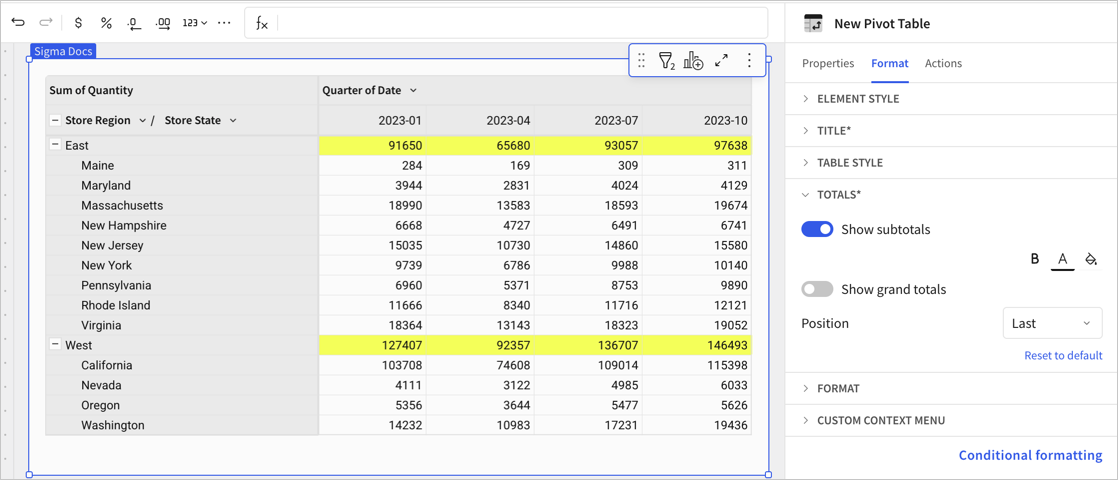
3. In the side panel, select **Format**, then click the **Totals** header to expand the section.
4. For **Show grand totals**, turn off the toggle.
All grand totals (the **Grand total** column and **Grand total** row) are removed from the pivot table.
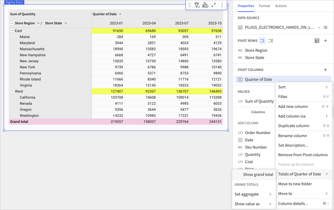
To hide or remove only the column-level grand total, do the following:
1. On the pivot table or in the editor panel, select the down arrow ( ) next to the column name. In this example, the **Quarter of Date** column.
2. In the dropdown menu, select **Totals of *Column Name***, then select **Show grand total** so that the checkmark disappears.
The **Grand total** column is removed from the pivot table.
### Hide parent row totals
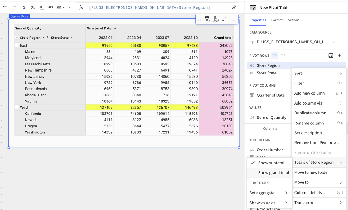
To hide or remove only the row-level grand total, do the following:
1. On the pivot table or in the editor panel, select the down arrow () next to the column name. In this example, the **Store Region** column.
2. In the dropdown menu, select **Totals of *Column Name***, then select **Show grand total** so that the checkmark disappears.
The **Grand total** row is removed from the pivot table.
### Hide subtotals
To hide or remove subtotals in a pivot table, do the following:
1. Start customizing a workbook or open it for editing.
2. Select the pivot table that you want to modify.
3. In the side panel, select **Format**, then click the **Totals** header to expand the section.
4. For **Show subtotals**, turn off the toggle.
All subtotals are removed from the pivot table. In this example, the **Total** row for each store region is removed.
If your pivot table displays rows as a single column and the rows are collapsed, hiding subtotals removes the total values from the pivot table:
You can also hide a specific subtotal level by deselecting **Show subtotals** in the column menu for the child pivot row. In this example, open the column menu for the **Store Region** column to hide the subtotal for all store states in each region.
## Customize totals and subtotals
Build more flexible reports by customizing the formula used to calculate totals and subtotals for grouped tables and pivot tables. Choose to set a different aggregate or write a custom formula to set a custom total or custom subtotal. You can also [customize the labels](#customize-total-labels) used for totals and subtotals, even if you don't customize the aggregate formula.
### Change aggregate of a subtotal
To change the aggregate of a subtotal in a pivot table or grouped table, such as from calculating a Sum() to an Avg(), do the following:
Before you start, make sure that the totals that you want to adjust are visible. See [Show and hide totals in a pivot table](#show-and-hide-totals-in-a-pivot-table) or [Show totals in a grouped table](/docs/create-and-manage-tables#show-totals-in-a-grouped-table).
1. Select a pivot table or grouped tables with totals.
2. For a subtotal or total, locate and select the total row or column.
3. Do one of the following:
* Right-click any cell in the totals row or column to open the context menu.
* For the relevant pivot row, column, or higher-level table grouping column, click the down arrow () to open the column menu.
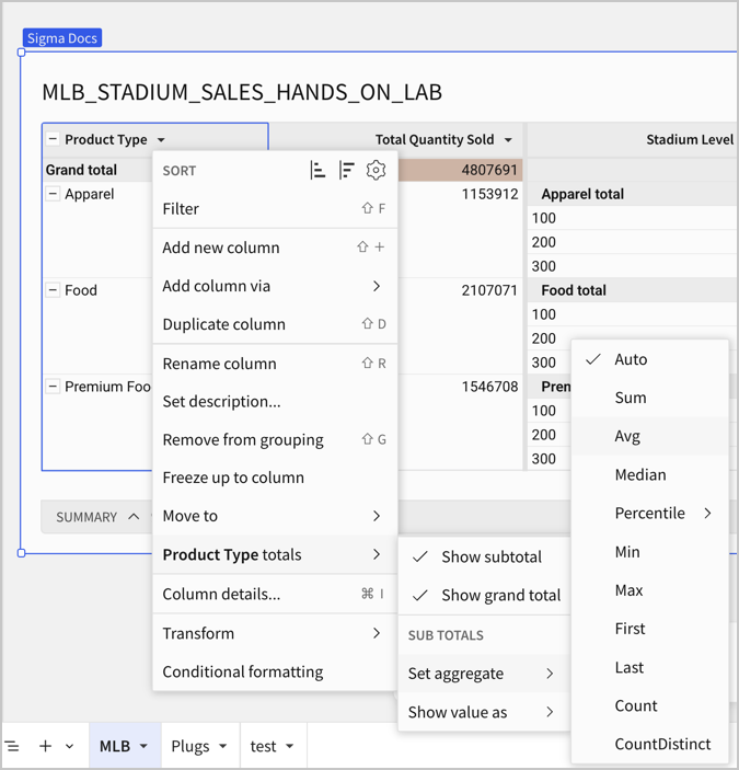
4. Select ***``* totals** , then choose **Set aggregate** and select the relevant aggregate function. The default is **Auto** (Sum).
The table updates to reflect the change:
#### Example: Customize grouped table subtotals
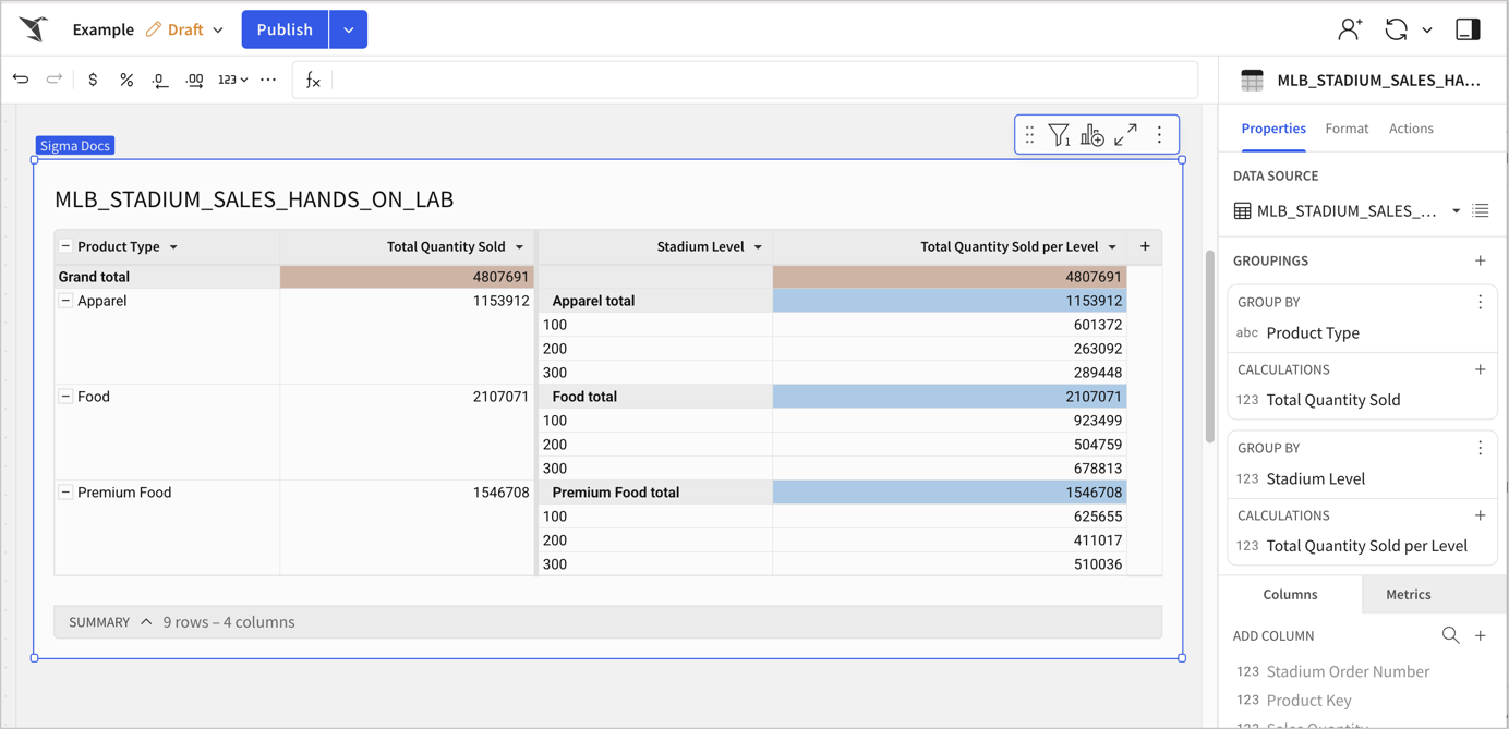
For example, if you have a grouped table that shows sales for specific product types in different stadium levels throughout a baseball season, you can set the subtotals for each stadium level to show the average sales, but keep the grand total as a sum.
1. Add a table to your workbook and use the MLB\_STADIUM\_SALES\_HANDS\_ON\_LAB table as your data source.
2. Configure the grouped table:
1. Create one grouping with the *Product Type* column and a calculation of *Sales Quantity*, which auto-aggregates to *Sum of Sales Quantity*. Rename the column *Total Quantity Sold*.
2. Add a second grouping with the *Stadium Level* column and a calculation of *Sales Quantity*, which auto-aggregates to *Sum of Sales Quantity*. Rename the column *Total Quantity Sold per Level*.
3. Hide the ungrouped columns.
3. Right-click a table cell to open the context menu, then choose **Show all totals**.
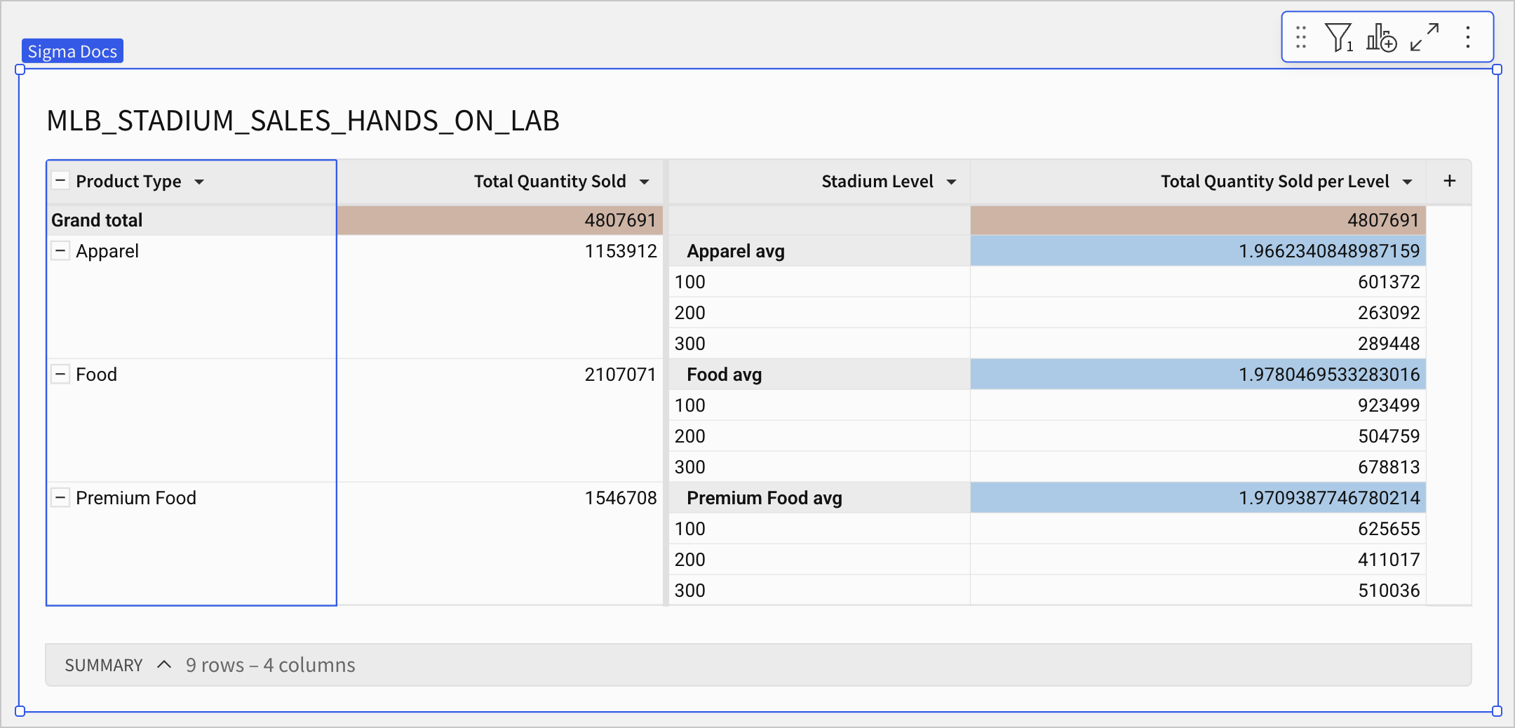
In this example, subtotals are highlighted in blue and grand total cells in brown using conditional formatting, and a filter limits the number of product types visible.
The grouped table looks something like the following:
4. Change the subtotal for each product type to calculate an average amount of sales, instead of a sum:
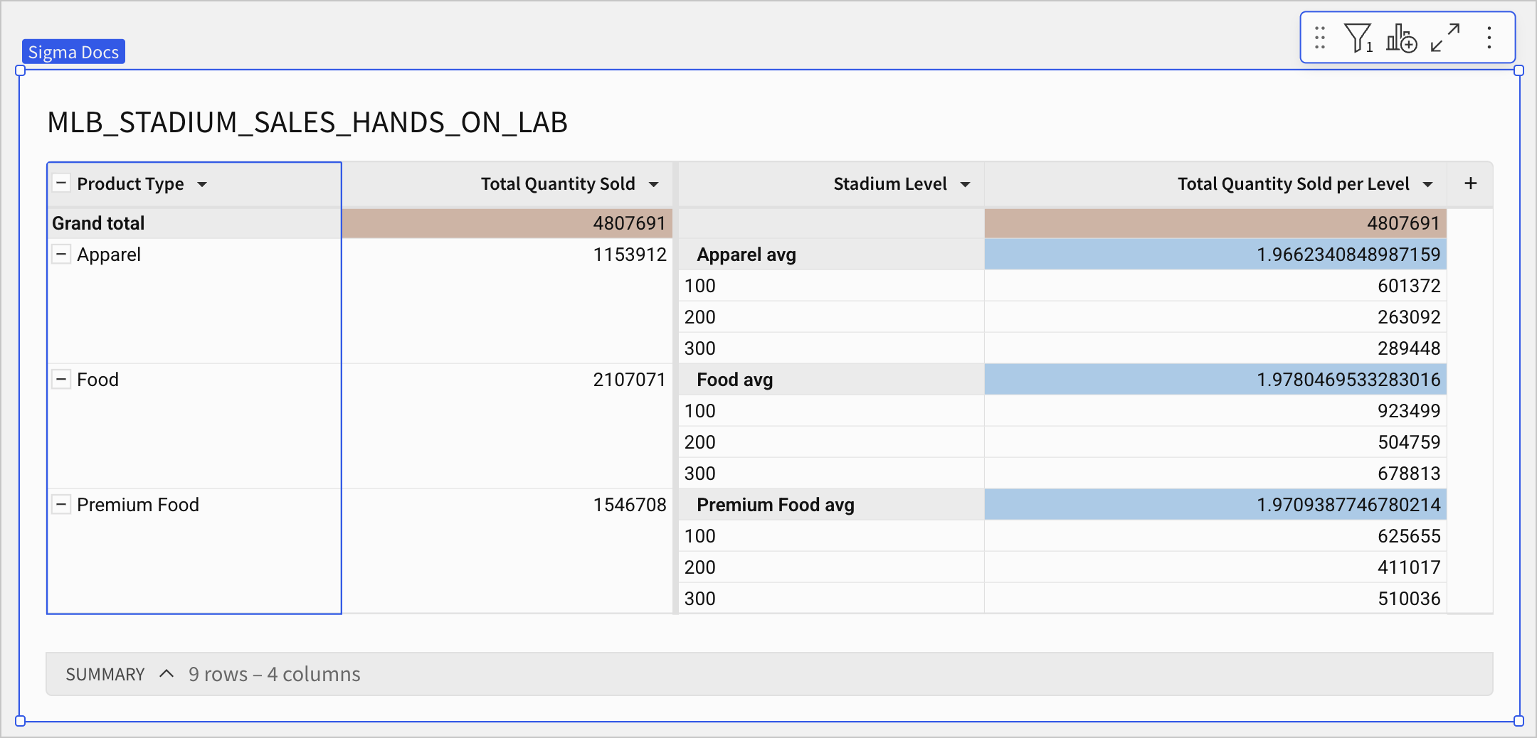
1. Click the down arrow () for the *Product Type* column to open the column menu, or right-click any cell in the totals row to open the context menu.
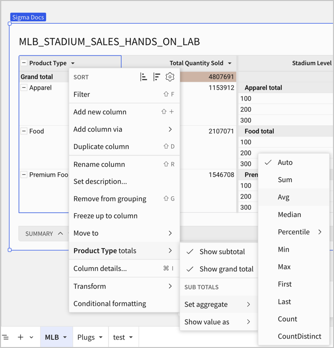
2. Select ***``* totals**, then choose **Set aggregate** and select the **Avg** aggregate function. The default is **Auto** (Sum).
The subtotal values and labels update accordingly:
5. \[optional] Modify the label for the *Product Type* subtotals. Double click on the total label to update it to *Average Sales Volume Per Purchase*. All labels for the subtotal update.
### Write a custom formula for a subtotal or grand total
To write a custom formula to calculate a subtotal or grand total, do the following:
Before you start, make sure that the totals that you want to adjust are visible. See [Show and hide totals in a pivot table](#show-and-hide-totals-in-a-pivot-table) or [Show totals in a grouped table](/docs/create-and-manage-tables#show-totals-in-a-grouped-table).
1. Locate the total row or column that you want to customize.
2. In the total row or column, select a cell to view the formula in the formula bar.
![Pivot table with the first values cell in the grand total row selected and showing a formula of Sum(\[Sales Quantity\]) in the formula bar](https://files.buildwithfern.com/sigma.docs.buildwithfern.com/8b90aa90cfcc2eab5425476de55edbbbe508afe57df58dc4f6eb3d511ce45eea/assets/docs-images/6ebec90d4074d31ab021d4e20e2d1e6b3d0b921feae468f0bfc73539d656479e-cs-pivot-formula.png)
3. Update the formula in the formula bar.
For example, to calculate the total for all product types for each *Stadium Level* but remove the minimum performing product type from the grand total, replace `Sum([Quantity])` with `Sum([Quantity]) - Min([Sum of Quantity (Parent Row Total)])`.
Your formula must apply to an aggregated value, not a top-level value, otherwise it might show unaggregated results.
The formula updates for all *Stadium Level* grand totals and the grand total label changes to *Custom grand total*.
![MLB Sales pivot table with the first cell in the Custom grand total row selected, showing the formula Sum(\[Sales Quantity\]) - Min(\[Total Sales Volume (Parent Row Total)\]) in the formula bar.](https://files.buildwithfern.com/sigma.docs.buildwithfern.com/3666a122dfb4519db6eca2ef3144e308fd2dcebf808da12dbc800319330282e4/assets/docs-images/775fdf901c6924bd9520d12b6abe90ebb8b95e8ec0799047a199552c270792d6-cs-pivot-end.png)
4. \[optional] Modify the label for the total row. See [Customize total labels](#customize-total-labels).
#### Example: Customize pivot table grand totals
For example, if you have a pivot table that shows sales for specific product types and product lines in different levels of a baseball stadium, you can set the grand total to a formula that removes the sales for the lowest-performing product type for a given stadium level, to see how overall sales would be affected if you stopped selling a given product type in a specific stadium level.
1. Add a pivot table to your workbook and use the MLB\_STADIUM\_SALES\_HANDS\_ON\_LAB table as your data source
2. Configure your pivot table like follows:
1. Add the *Product Type* and *Product Line* columns as pivot rows.
2. Add the *Stadium Level* column as a pivot column.
3. Add the *Sales Quantity* column as a pivot value, which is automatically aggregated as *Sum of Sales Quantity*. Rename the column *Total Sales Volume*.
4. Set the display of your pivot table to **Display as separate columns**.
In this example, subtotals are highlighted in blue and grand total cells in brown using conditional formatting, and a filter limits the number of product types visible.
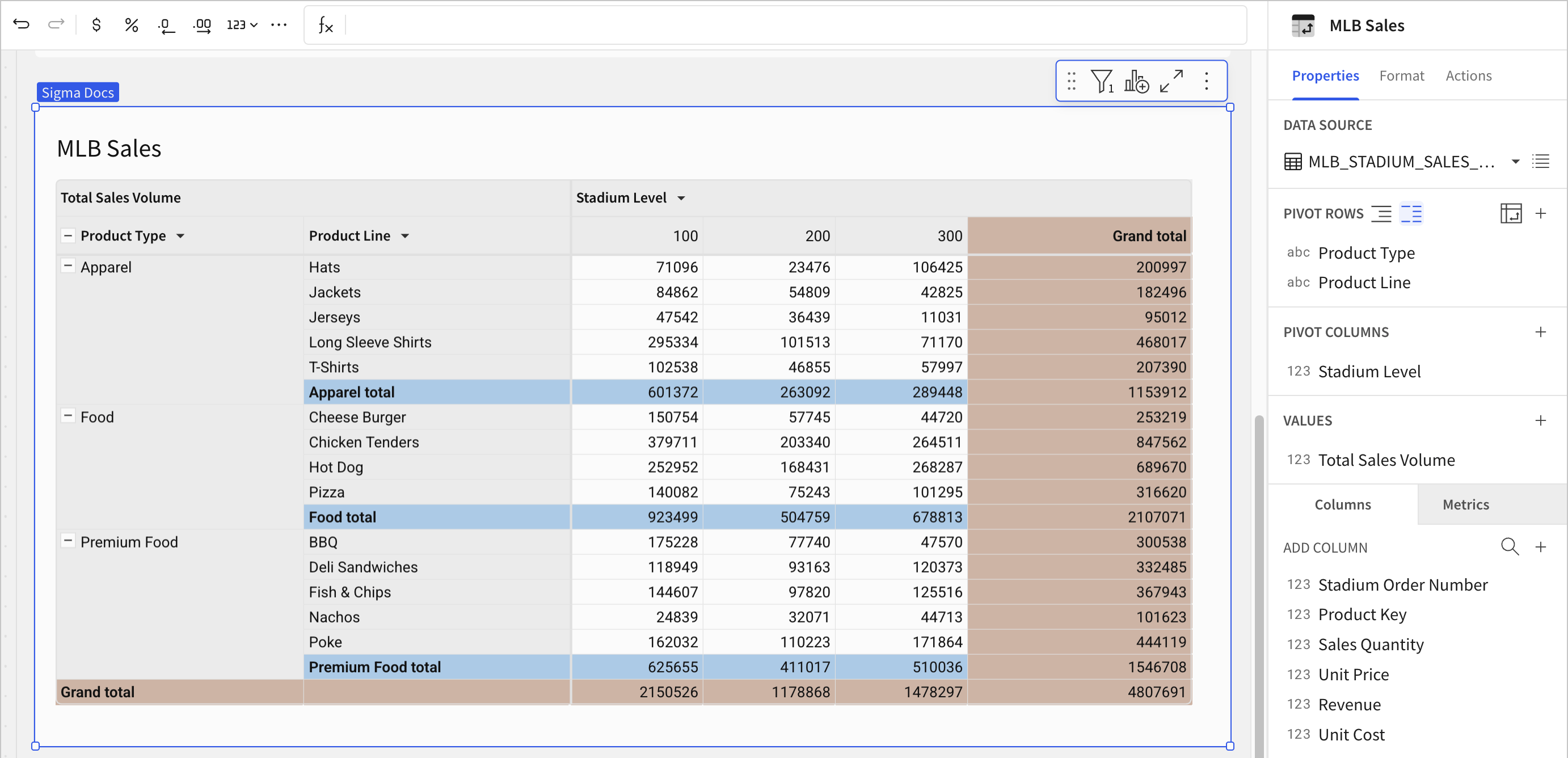
3. To change the grand total to a custom formula that removes sales for the lowest-performing product line for each stadium level, locate the grand total row.
The grand total column calculates the total sales volume for each product line across all stadium levels, while the grand total row calculates the total sales volume for all product types for each stadium level.
4. Select a cell in the grand total row, then modify the formula from `Sum([Sales Quantity])` to `Sum([Sales Quantity]) - Min([Total Sales Volume (Parent Row Total)])`.
![MLB Sales pivot table with the first cell in the Grand total row selected, showing the formula Sum(\[Sales Quantity\]) in the formula bar.](https://files.buildwithfern.com/sigma.docs.buildwithfern.com/8b90aa90cfcc2eab5425476de55edbbbe508afe57df58dc4f6eb3d511ce45eea/assets/docs-images/6ebec90d4074d31ab021d4e20e2d1e6b3d0b921feae468f0bfc73539d656479e-cs-pivot-formula.png)
The grand total values update for the row and the label updates to *Custom grand total*.
![MLB Sales pivot table with the Custom grand total row at the bottom, showing the formula Sum(\[Sales Quantity\]) - Min(\[Total Sales Volume (Parent Row Total)\]) in the formula bar.](https://files.buildwithfern.com/sigma.docs.buildwithfern.com/3666a122dfb4519db6eca2ef3144e308fd2dcebf808da12dbc800319330282e4/assets/docs-images/775fdf901c6924bd9520d12b6abe90ebb8b95e8ec0799047a199552c270792d6-cs-pivot-end.png)
### Customize total labels
You can customize the label for a subtotal or grand total in a table or pivot table:
1. Locate the total label that you want to rename on the table or pivot table.
2. Double-click the label to make it editable, then enter a new label.
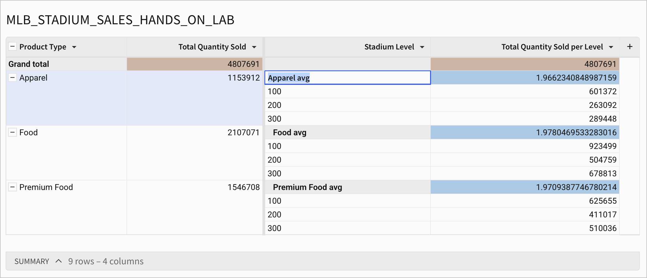
If you change the label for a subtotal, all subtotal labels change for that level and value combination.
3. Press enter on your keyboard, or click outside of the cell, to save the new label.
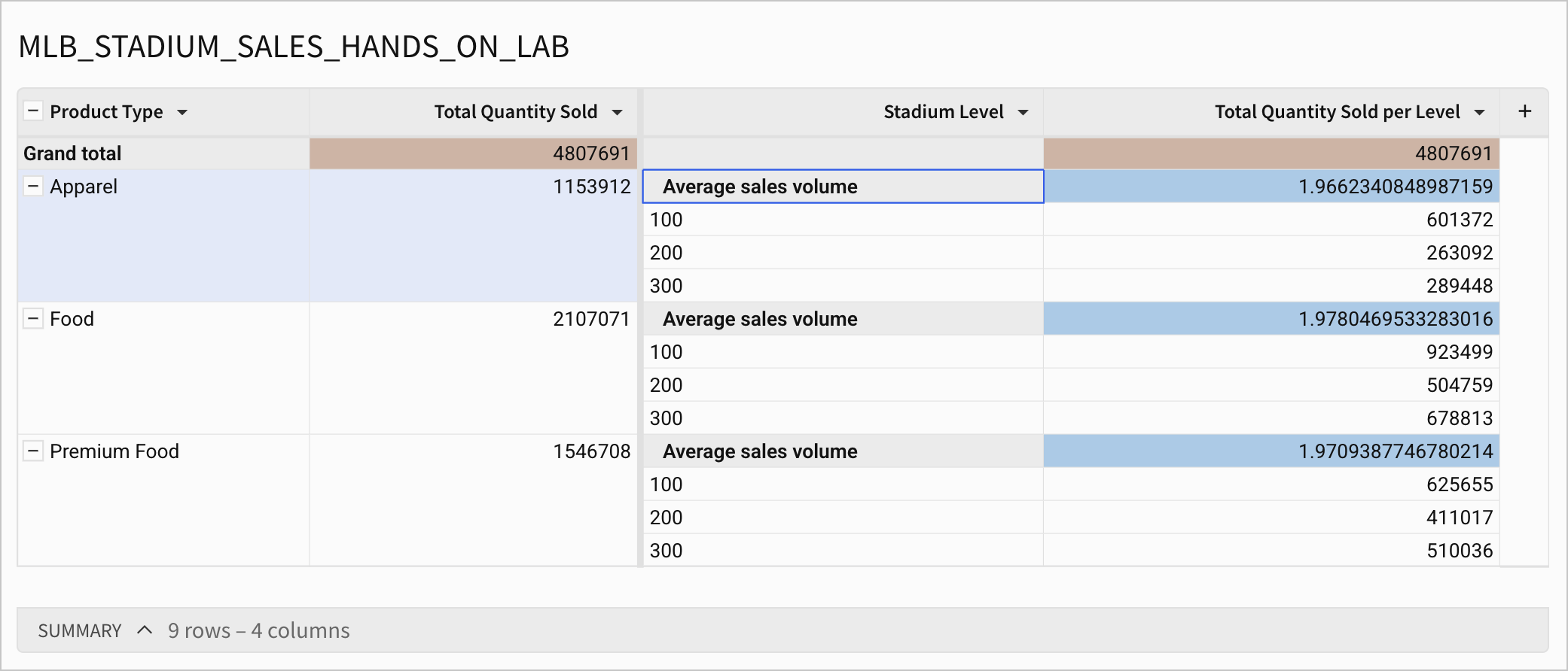
To revert to the default label for a total or subtotal, remove the existing label. Double-click the label and delete the existing label, then press enter to save your changes.
### Limitations when customizing totals and subtotals
* Renamed subtotal and grand total labels are not updated downstream. Child tables created from a pivot table or grouped table with custom formulas for totals display the original column names. Any formulas, such as summary metrics, that reference the total or subtotal values must instead reference the original column names:
* *\<Values Column Name> (Parent Row Total)* for subtotals on a pivot row.
* *\<Values Column Name> (Row Total)* for grand totals of a pivot row.
* *\<Values Column Name> (Parent Column Total)* for subtotals of a pivot column.
* *\<Values Column Name> (Column Total)* for grand totals of a pivot column.
* *\<Values Column Name> (Grand Total)* for the grand total of the value for both rows and columns for a pivot table or grouped table.
* After customizing a subtotal formula, cells where subtotals interact might be blank if the intersecting total does not make sense. For example, if one subtotal calculates an average and the other subtotal calculates the maximum value:
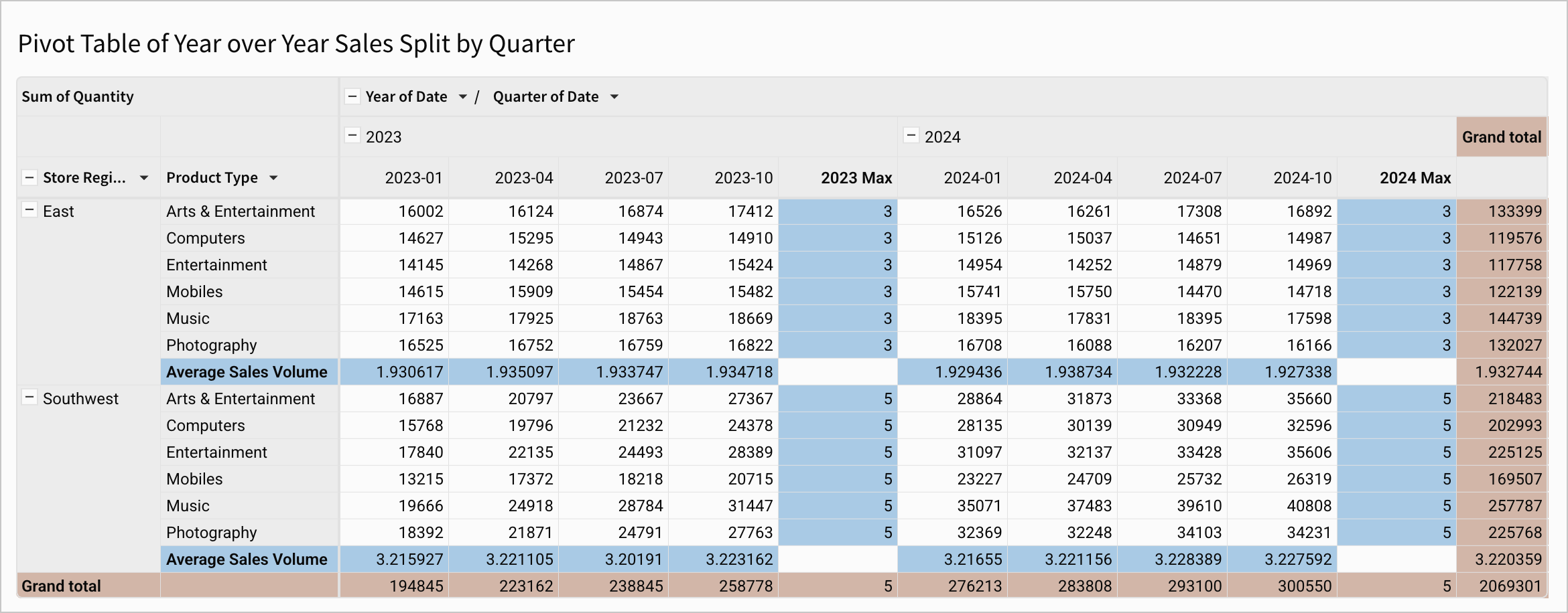
## Tutorial: Calculate a percentage for subtotals in a pivot table
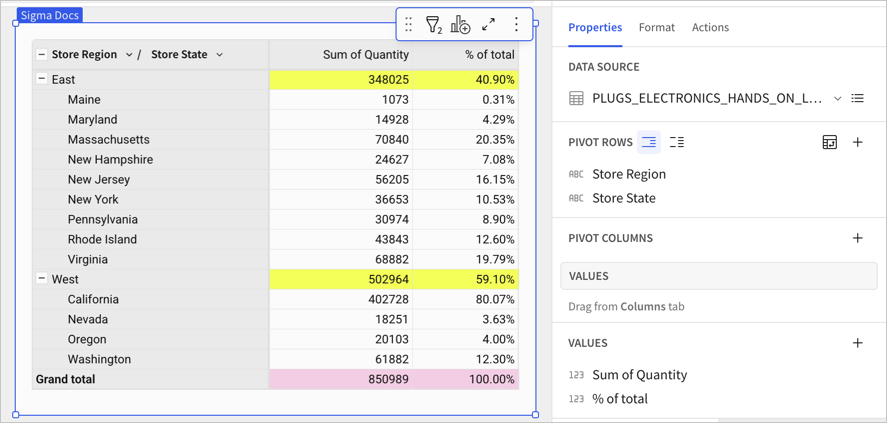
In this example, calculate the percent of total units sold in a given region. This example uses the PLUGS\_ELECTRONICS\_HANDS\_ON\_LAB\_DATA table included in the Sigma Sample Database.
Start with a pivot table with pivot rows **Store Region** and **Store State** and an aggregate value of **Sum of Quantity**.
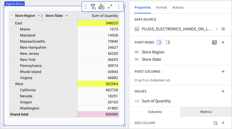
To calculate the percentage of total units sold, add a new column to the pivot table:
1. In the editor panel, in the **Values** header, click **Add calculation...** (**+**).
2. Select **Add new column**.
3. In the formula bar for the new column, enter:
```
[Sum of Quantity (Row Total)] / [Sum of Quantity (Parent Row Total)]
```
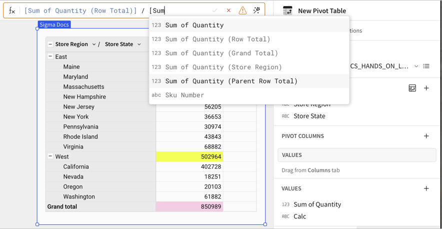
4. Press **Enter** or click the checkmark to save the formula.
5. To format the calculated column as a percentage, in the workbook toolbar, click **Format as percent** (%).
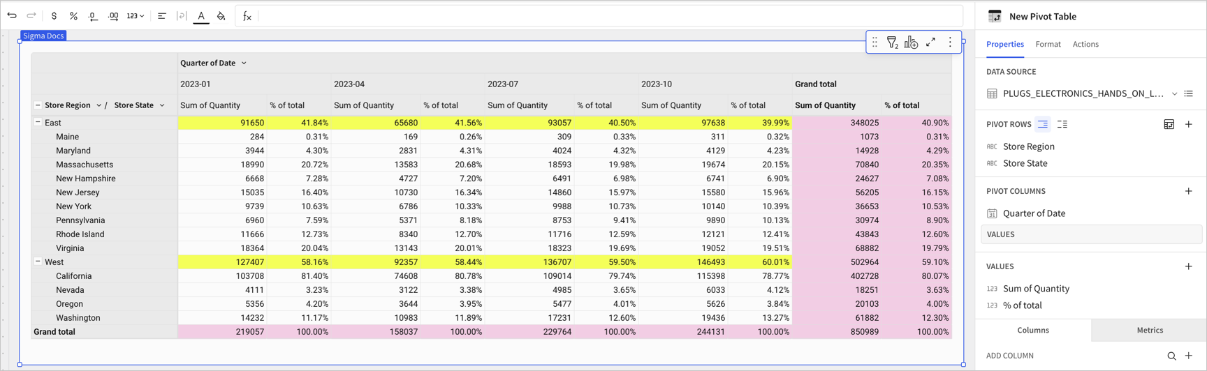
The result appears as follows:
## Tutorial: Calculate a percentage for row subtotals
In this tutorial, calculate the percent of total state retail sales broken down by region and sales quarter.
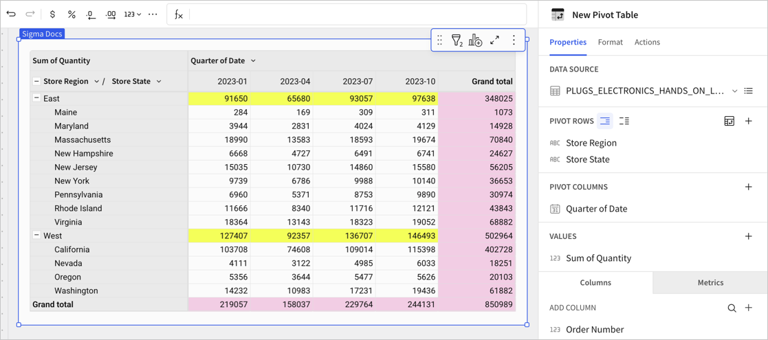
Start with a pivot table with pivot rows **Store Region** and **Store State**, a pivot column of **Date**, truncated to display **Quarter of Date**, and an aggregate value of **Sum of Quantity**.
1. In the editor panel, in the **Values** header, click **Add calculation...** (**+**).
2. Select **Add new column**.
3. In the formula bar for the new column, enter:
```
[Sum of Quantity] / [Sum of Quantity (Parent Row Total)]
```
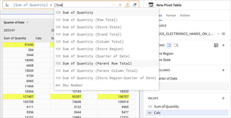
4. Press **Enter** or click the checkmark to save the formula.
5. To format the calculated column as a percentage, in the workbook toolbar, click **Format as percent** (%).
The result appears as follows:
## Related resources
* [Working with pivot tables](/docs/working-with-pivot-tables)
* [Format pivot table totals](/docs/format-pivot-table-totals)
* [PercentOfTotal](/docs/percentoftotal)
* [Subtotal](/docs/subtotal)
) next to the column name. In this example, the **Quarter of Date** column.
2. In the dropdown menu, select **Totals of *Column Name***, then select **Show grand total** so that the checkmark disappears.
The **Grand total** column is removed from the pivot table.

### Hide parent row totals
To hide or remove only the row-level grand total, do the following:
1. On the pivot table or in the editor panel, select the down arrow () next to the column name. In this example, the **Store Region** column.
2. In the dropdown menu, select **Totals of *Column Name***, then select **Show grand total** so that the checkmark disappears.
The **Grand total** row is removed from the pivot table.

### Hide subtotals
To hide or remove subtotals in a pivot table, do the following:
1. Start customizing a workbook or open it for editing.
2. Select the pivot table that you want to modify.
3. In the side panel, select **Format**, then click the **Totals** header to expand the section.
4. For **Show subtotals**, turn off the toggle.
All subtotals are removed from the pivot table. In this example, the **Total** row for each store region is removed.

If your pivot table displays rows as a single column and the rows are collapsed, hiding subtotals removes the total values from the pivot table:

You can also hide a specific subtotal level by deselecting **Show subtotals** in the column menu for the child pivot row. In this example, open the column menu for the **Store Region** column to hide the subtotal for all store states in each region.
## Customize totals and subtotals
Build more flexible reports by customizing the formula used to calculate totals and subtotals for grouped tables and pivot tables. Choose to set a different aggregate or write a custom formula to set a custom total or custom subtotal. You can also [customize the labels](#customize-total-labels) used for totals and subtotals, even if you don't customize the aggregate formula.
### Change aggregate of a subtotal
To change the aggregate of a subtotal in a pivot table or grouped table, such as from calculating a Sum() to an Avg(), do the following:
Before you start, make sure that the totals that you want to adjust are visible. See [Show and hide totals in a pivot table](#show-and-hide-totals-in-a-pivot-table) or [Show totals in a grouped table](/docs/create-and-manage-tables#show-totals-in-a-grouped-table).
1. Select a pivot table or grouped tables with totals.
2. For a subtotal or total, locate and select the total row or column.
3. Do one of the following:
* Right-click any cell in the totals row or column to open the context menu.
* For the relevant pivot row, column, or higher-level table grouping column, click the down arrow () to open the column menu.
4. Select ***``* totals** , then choose **Set aggregate** and select the relevant aggregate function. The default is **Auto** (Sum).

The table updates to reflect the change:

#### Example: Customize grouped table subtotals
For example, if you have a grouped table that shows sales for specific product types in different stadium levels throughout a baseball season, you can set the subtotals for each stadium level to show the average sales, but keep the grand total as a sum.
1. Add a table to your workbook and use the MLB\_STADIUM\_SALES\_HANDS\_ON\_LAB table as your data source.
2. Configure the grouped table:
1. Create one grouping with the *Product Type* column and a calculation of *Sales Quantity*, which auto-aggregates to *Sum of Sales Quantity*. Rename the column *Total Quantity Sold*.
2. Add a second grouping with the *Stadium Level* column and a calculation of *Sales Quantity*, which auto-aggregates to *Sum of Sales Quantity*. Rename the column *Total Quantity Sold per Level*.
3. Hide the ungrouped columns.
3. Right-click a table cell to open the context menu, then choose **Show all totals**.
In this example, subtotals are highlighted in blue and grand total cells in brown using conditional formatting, and a filter limits the number of product types visible.
The grouped table looks something like the following:

4. Change the subtotal for each product type to calculate an average amount of sales, instead of a sum:
1. Click the down arrow () for the *Product Type* column to open the column menu, or right-click any cell in the totals row to open the context menu.

2. Select ***``* totals**, then choose **Set aggregate** and select the **Avg** aggregate function. The default is **Auto** (Sum).
The subtotal values and labels update accordingly:

5. \[optional] Modify the label for the *Product Type* subtotals. Double click on the total label to update it to *Average Sales Volume Per Purchase*. All labels for the subtotal update.
### Write a custom formula for a subtotal or grand total
To write a custom formula to calculate a subtotal or grand total, do the following:
Before you start, make sure that the totals that you want to adjust are visible. See [Show and hide totals in a pivot table](#show-and-hide-totals-in-a-pivot-table) or [Show totals in a grouped table](/docs/create-and-manage-tables#show-totals-in-a-grouped-table).
1. Locate the total row or column that you want to customize.
2. In the total row or column, select a cell to view the formula in the formula bar.
![Pivot table with the first values cell in the grand total row selected and showing a formula of Sum(\[Sales Quantity\]) in the formula bar](https://files.buildwithfern.com/sigma.docs.buildwithfern.com/8b90aa90cfcc2eab5425476de55edbbbe508afe57df58dc4f6eb3d511ce45eea/assets/docs-images/6ebec90d4074d31ab021d4e20e2d1e6b3d0b921feae468f0bfc73539d656479e-cs-pivot-formula.png)
3. Update the formula in the formula bar.
For example, to calculate the total for all product types for each *Stadium Level* but remove the minimum performing product type from the grand total, replace `Sum([Quantity])` with `Sum([Quantity]) - Min([Sum of Quantity (Parent Row Total)])`.
Your formula must apply to an aggregated value, not a top-level value, otherwise it might show unaggregated results.
The formula updates for all *Stadium Level* grand totals and the grand total label changes to *Custom grand total*.
![MLB Sales pivot table with the first cell in the Custom grand total row selected, showing the formula Sum(\[Sales Quantity\]) - Min(\[Total Sales Volume (Parent Row Total)\]) in the formula bar.](https://files.buildwithfern.com/sigma.docs.buildwithfern.com/3666a122dfb4519db6eca2ef3144e308fd2dcebf808da12dbc800319330282e4/assets/docs-images/775fdf901c6924bd9520d12b6abe90ebb8b95e8ec0799047a199552c270792d6-cs-pivot-end.png)
4. \[optional] Modify the label for the total row. See [Customize total labels](#customize-total-labels).
#### Example: Customize pivot table grand totals
For example, if you have a pivot table that shows sales for specific product types and product lines in different levels of a baseball stadium, you can set the grand total to a formula that removes the sales for the lowest-performing product type for a given stadium level, to see how overall sales would be affected if you stopped selling a given product type in a specific stadium level.
1. Add a pivot table to your workbook and use the MLB\_STADIUM\_SALES\_HANDS\_ON\_LAB table as your data source
2. Configure your pivot table like follows:
1. Add the *Product Type* and *Product Line* columns as pivot rows.
2. Add the *Stadium Level* column as a pivot column.
3. Add the *Sales Quantity* column as a pivot value, which is automatically aggregated as *Sum of Sales Quantity*. Rename the column *Total Sales Volume*.
4. Set the display of your pivot table to **Display as separate columns**.
In this example, subtotals are highlighted in blue and grand total cells in brown using conditional formatting, and a filter limits the number of product types visible.

3. To change the grand total to a custom formula that removes sales for the lowest-performing product line for each stadium level, locate the grand total row.
The grand total column calculates the total sales volume for each product line across all stadium levels, while the grand total row calculates the total sales volume for all product types for each stadium level.
4. Select a cell in the grand total row, then modify the formula from `Sum([Sales Quantity])` to `Sum([Sales Quantity]) - Min([Total Sales Volume (Parent Row Total)])`.
![MLB Sales pivot table with the first cell in the Grand total row selected, showing the formula Sum(\[Sales Quantity\]) in the formula bar.](https://files.buildwithfern.com/sigma.docs.buildwithfern.com/8b90aa90cfcc2eab5425476de55edbbbe508afe57df58dc4f6eb3d511ce45eea/assets/docs-images/6ebec90d4074d31ab021d4e20e2d1e6b3d0b921feae468f0bfc73539d656479e-cs-pivot-formula.png)
The grand total values update for the row and the label updates to *Custom grand total*.
![MLB Sales pivot table with the Custom grand total row at the bottom, showing the formula Sum(\[Sales Quantity\]) - Min(\[Total Sales Volume (Parent Row Total)\]) in the formula bar.](https://files.buildwithfern.com/sigma.docs.buildwithfern.com/3666a122dfb4519db6eca2ef3144e308fd2dcebf808da12dbc800319330282e4/assets/docs-images/775fdf901c6924bd9520d12b6abe90ebb8b95e8ec0799047a199552c270792d6-cs-pivot-end.png)
### Customize total labels
You can customize the label for a subtotal or grand total in a table or pivot table:
1. Locate the total label that you want to rename on the table or pivot table.
2. Double-click the label to make it editable, then enter a new label.

If you change the label for a subtotal, all subtotal labels change for that level and value combination.
3. Press enter on your keyboard, or click outside of the cell, to save the new label.

To revert to the default label for a total or subtotal, remove the existing label. Double-click the label and delete the existing label, then press enter to save your changes.
### Limitations when customizing totals and subtotals
* Renamed subtotal and grand total labels are not updated downstream. Child tables created from a pivot table or grouped table with custom formulas for totals display the original column names. Any formulas, such as summary metrics, that reference the total or subtotal values must instead reference the original column names:
* *\<Values Column Name> (Parent Row Total)* for subtotals on a pivot row.
* *\<Values Column Name> (Row Total)* for grand totals of a pivot row.
* *\<Values Column Name> (Parent Column Total)* for subtotals of a pivot column.
* *\<Values Column Name> (Column Total)* for grand totals of a pivot column.
* *\<Values Column Name> (Grand Total)* for the grand total of the value for both rows and columns for a pivot table or grouped table.
* After customizing a subtotal formula, cells where subtotals interact might be blank if the intersecting total does not make sense. For example, if one subtotal calculates an average and the other subtotal calculates the maximum value:

## Tutorial: Calculate a percentage for subtotals in a pivot table
In this example, calculate the percent of total units sold in a given region. This example uses the PLUGS\_ELECTRONICS\_HANDS\_ON\_LAB\_DATA table included in the Sigma Sample Database.
Start with a pivot table with pivot rows **Store Region** and **Store State** and an aggregate value of **Sum of Quantity**.

To calculate the percentage of total units sold, add a new column to the pivot table:
1. In the editor panel, in the **Values** header, click **Add calculation...** (**+**).
2. Select **Add new column**.
3. In the formula bar for the new column, enter:
```
[Sum of Quantity (Row Total)] / [Sum of Quantity (Parent Row Total)]
```

4. Press **Enter** or click the checkmark to save the formula.
5. To format the calculated column as a percentage, in the workbook toolbar, click **Format as percent** (%).
The result appears as follows:

## Tutorial: Calculate a percentage for row subtotals
In this tutorial, calculate the percent of total state retail sales broken down by region and sales quarter.
Start with a pivot table with pivot rows **Store Region** and **Store State**, a pivot column of **Date**, truncated to display **Quarter of Date**, and an aggregate value of **Sum of Quantity**.

1. In the editor panel, in the **Values** header, click **Add calculation...** (**+**).
2. Select **Add new column**.
3. In the formula bar for the new column, enter:
```
[Sum of Quantity] / [Sum of Quantity (Parent Row Total)]
```

4. Press **Enter** or click the checkmark to save the formula.
5. To format the calculated column as a percentage, in the workbook toolbar, click **Format as percent** (%).
The result appears as follows:

## Related resources
* [Working with pivot tables](/docs/working-with-pivot-tables)
* [Format pivot table totals](/docs/format-pivot-table-totals)
* [PercentOfTotal](/docs/percentoftotal)
* [Subtotal](/docs/subtotal)